Code360 powered by Coding Ninjas X Naukri.com. Code360 powered by Coding Ninjas X Naukri.com
Table of contents
1.
Introduction
1.1.
For example:
2.
0-1 BFS Algorithm
2.1.
Basic code of 0-1 BFS(C++)
3.
Code in C++
3.1.
C++
3.2.
Complexity Analysis
4.
Implementation of 0-1 BFS on Java and Python3
4.1.
Java
4.2.
Python
5.
Why to use 0-1 BFS Algorithm?
6.
Frequently asked questions
6.1.
Can we use Dijkstra for this problem? 
6.2.
What is the BFS sequence?
6.3.
What is the time complexity of the BFS algorithm?
7.
Conclusion
Last Updated: Jul 3, 2024
Easy

0-1 BFS

Author Sandeep kamila
2 upvotes

Introduction

Welcome to our blog on the topic 0-1 BFS (Breadth-First Search)! In this comprehensive blog, we delve into the intricacies and applications of this variant of the classic BFS algorithm. We will understand what it is and how it can be implemented.

0-1 BFS

For example:


In the unweighted graph above, the shortest distance between the source node (1) and node (7) will be node1→ node3→ node4→node7 having 3 edges.                       

For the shortest path in a weighted graph, we consider the path having the minimum sum of their edge weights. 


For example:
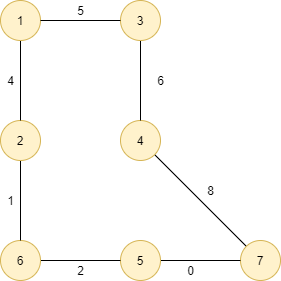
 

In the unweighted graph given above, there are two paths from the source node(1) to node(7):

  1. node1→ node3→ node4→node7 has a total edge weight of 19 units.   
     
  2. node1→ node2→ node6→node5→node7 has a total edge weight of 7 units.

So, the shortest distance between the source node (1) and node (7) is node1→node2→ node6→node5→node7 having a total edge weight of 7 units.

We can use the Dijkstra algorithm for finding the shortest path in a weighted graph, which runs in O( E + VlogV ) time, but we can find a better solution if the weights are more constrained. This article will look at a better approach for solving the shortest path problem using a double-ended queue (Deque) called the 0-1 BFS algorithm, which works only when all edge weights are 0 or 1.

Also read, Euclid GCD Algorithm

0-1 BFS Algorithm

It is named 0-1 BFS because it only works for graphs with edge weights of 0 or 1. This type of BFS is used to calculate the shortest distance between the source node to all other vertices where the edges have weights of 0 or 1.

We will use deque (double-ended queue) in 0-1 BFS, which allows us to insert or delete elements from the front and back in O(1) time complexity.

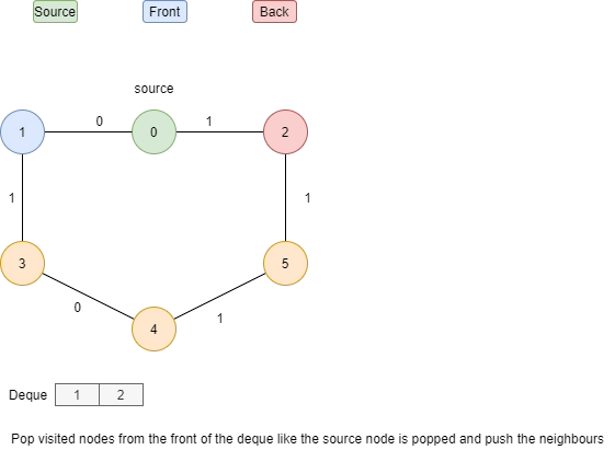
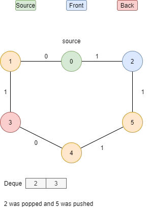
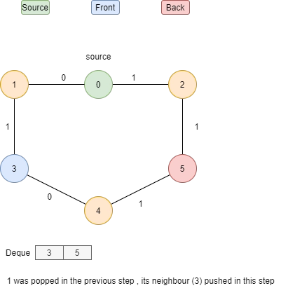
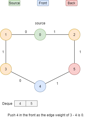
  1. Traverse through all the nodes of the graph (source node will be pushed in the front of the deque, and then its neighbour nodes are pushed after popping the source node).
  2. Check the weight of all edges of the graph.
  3. Push the nodes into the deque, i.e. if the weight is 0, push it in the front of the deque else, push it to the back of the deque.
  4. Print the sum of the weight of edges, making the shortest path from the source node to other nodes.

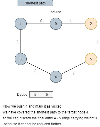
Let’s understand this algorithm with an example:
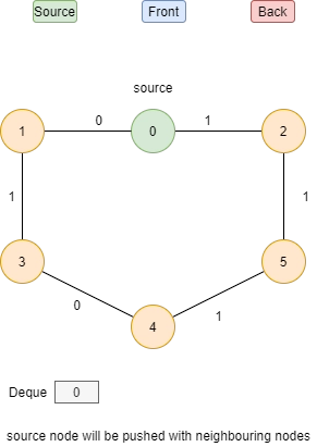


Basic code of 0-1 BFS(C++)

void ZeroOneBfs (int source)
{
    deque <int> deq;  
   
    deq.push_back( source);

    dist[ source ] = 0;

    while ( !deq.empty ())
    {
        int v = deq.front( );
        deq.pop_front();
        for ( int i = 0 ; i < edges[v].size(); i++)
        {

            if (dist[ edges[ v ][ i ].first ] > dist[ v ] + edges[ v ][ i ].second )
            {
                dist[ edges[ v ][ i ].first ] = dist[ v ] + edges[ v ][ i ].second;

                if (edges[ v ][ i ].second == 0)
                {
                    deq.push_front( edges[ v ][ i ].first);
                }
                else
                {
                    deq.push_back( edges[ v ][ i ].first);

                }
            }
        }
    }
}

Code in C++

Let’s have a look at the implementation of the above approach:

  • C++

C++

#include <bits/stdc++.h>
#define V 6
using namespace std;

struct node {
int no, weight; // no denoted the node and weight denoted the weight of edges
};

vector <node> Edges[V]; // to store edges

void ZeroOneBFS(int src) {

int dist[V]; 

for (int i = 0; i < V; i++)
dist[i] = INT_MAX;

deque <int> Q;

dist[src] = 0;  //distance from source to source is 0

Q.push_back(src);

while (!Q.empty()) {

int v = Q.front();

Q.pop_front();

for (int i = 0; i < Edges[v].size(); i++) {

if (dist[Edges[v][i].no] > dist[v] + Edges[v][i].weight) {

dist[Edges[v][i].no] = dist[v] + Edges[v][i].weight;

if (Edges[v][i].weight == 0)  //if 0 weight edge, store at front of deque

Q.push_front(Edges[v][i].no);
else
Q.push_back(Edges[v][i].no);  // if 1 weight edge, store at back of deque
}

}

}

for (int i = 0; i < V; i++)
cout << "Distance from the source node to " << i << ":" << "\t" << dist[i] << endl;
}

void insertEdge(int u, int v, int wt) {
Edges[u].push_back({v, wt});
Edges[v].push_back({u, wt});
}
int main() {
insertEdge(0, 1, 0);
insertEdge(0, 2, 1);
insertEdge(1, 3, 1);
insertEdge(3, 4, 0);
insertEdge(4, 5, 1);
insertEdge(5, 2, 1);

int src = 0;
ZeroOneBFS(src);
}

Output

Distance from the source node to 0: 0
Distance from the source node to 1: 0
Distance from the source node to 2: 1
Distance from the source node to 3: 1
Distance from the source node to 4: 1
Distance from the source node to 5: 2

Complexity Analysis

Time complexity

All nodes have been visited only once in this algorithm. As a result, the time complexity of 0-1 BFS is O(E + V), linear and faster than Dijkstra, which runs in O(E+VlogV).

Space complexity

As we store the graph in an adjacency list and maintain a deque and a distance array to store the distances of the nodes, the space complexity turns out to be O(V + E).

Read MoreTime Complexity of Sorting Algorithms, Graph Traversal Techniques in DFS BFS

Implementation of 0-1 BFS on Java and Python3

  • Java
  • Python

Java

import java.util.*;

class Main {
static int V = 6;
static ArrayList<Node>[] edges = new ArrayList[V];

static class Node {
int no, weight;

Node(int no, int weight) {
this.no = no;
this.weight = weight;
}
}

static void zeroOneBFS(int src) {
int[] dist = new int[V];
Arrays.fill(dist, Integer.MAX_VALUE);

Deque<Integer> Q = new ArrayDeque<>();

dist[src] = 0;
Q.addLast(src);

while (!Q.isEmpty()) {
int v = Q.pollFirst();

for (Node edge : edges[v]) {
if (dist[edge.no] > dist[v] + edge.weight) {
dist[edge.no] = dist[v] + edge.weight;
if (edge.weight == 0)
Q.addFirst(edge.no);
else
Q.addLast(edge.no);
}
}
}

for (int i = 0; i < V; i++)
System.out.println("Distance from the source node to " + i + ": " + dist[i]);
}

static void insertEdge(int u, int v, int wt) {
edges[u].add(new Node(v, wt));
edges[v].add(new Node(u, wt));
}

public static void main(String[] args) {
for (int i = 0; i < V; i++)
edges[i] = new ArrayList<>();

insertEdge(0, 1, 0);
insertEdge(0, 2, 1);
insertEdge(1, 3, 1);
insertEdge(3, 4, 0);
insertEdge(4, 5, 1);
insertEdge(5, 2, 1);

int src = 0;
zeroOneBFS(src);
}
}

Python

from collections import deque

V = 6
edges = [[] for _ in range(V)]

class Node:
def __init__(self, no, weight):
self.no = no
self.weight = weight

def zero_one_bfs(src):
dist = [float('inf')] * V
dist[src] = 0

Q = deque()
Q.append(src)

while Q:
v = Q.popleft()

for edge in edges[v]:
if dist[edge.no] > dist[v] + edge.weight:
dist[edge.no] = dist[v] + edge.weight
if edge.weight == 0:
Q.appendleft(edge.no)
else:
Q.append(edge.no)

for i in range(V):
print(f"Distance from the source node to {i}: {dist[i]}")

def insert_edge(u, v, wt):
edges[u].append(Node(v, wt))
edges[v].append(Node(u, wt))

if __name__ == "__main__":
insert_edge(0, 1, 0)
insert_edge(0, 2, 1)
insert_edge(1, 3, 1)
insert_edge(3, 4, 0)
insert_edge(4, 5, 1)
insert_edge(5, 2, 1)

src = 0
zero_one_bfs(src)

Why to use 0-1 BFS Algorithm?

The 0-1 BFS algorithm is utilized for its efficiency and versatility in solving shortest path problems in graphs with weighted edges of only 0 or 1. Here's why it's advantageous:

  • Efficiency: 0-1 BFS has a time complexity of O(V + E), where V is the number of vertices and E is the number of edges, making it highly efficient compared to other shortest path algorithms like Dijkstra's algorithm.
  • Optimality: In graphs where edges have weights restricted to 0 or 1, the 0-1 BFS algorithm always finds the shortest path from the source node to all other nodes, ensuring optimality in the shortest path solution.
  • Space Complexity: The space complexity of 0-1 BFS is O(V), which is relatively low compared to other algorithms like Dijkstra's, which can have a higher space complexity due to priority queues or heaps.
  • Simplicity: The algorithm is straightforward to implement and understand, requiring only a deque (double-ended queue) data structure for traversal.
  • Applications: 0-1 BFS finds applications in various domains such as routing algorithms in computer networks, grid-based pathfinding in games and robotics, and solving shortest path problems in graphs with binary weights, making it a versatile tool in algorithmic problem-solving.

Frequently asked questions

Can we use Dijkstra for this problem? 

Yes, we can find the shortest path in a weighted graph using Dijkstra; it runs with time complexity of O(E + V log V). 

What is the BFS sequence?

The breadth-First Search (BFS) algorithm traverses the graph in a breadthward motion and uses a queue data structure to get the next vertex to start a search when a dead end occurs in any iteration.

What is the time complexity of the BFS algorithm?

The time complexity of the BFS algorithm is O(V+E) when the adjacency list is used as every node is visited once and O(V 2) when the adjacency matrix is used.

Conclusion

So, this article discussed the shortest path in an unweighted and weighted graph, using the 0-1 BFS algorithm with an example and its code in the C++ programming language.

If you are a beginner in coding and want to learn DSA, you can look for our guided path for DSA, which is free! 

In case of any comments or suggestions, feel free to post them in the comments section.

Live masterclass