Do you think IIT Guwahati certified course can help you in your career?
Introduction
First, let us get to know the history of the AlexNet. The AlexNet CNN architecture11 won the 2012 ImageNet ILSVRC challenge by a large margin: it achieved a 17% top-5 error rate while the second-best achieved only 26%! It was developed by Alex Krizhevsky, Ilya Sutskever, and Geoffrey Hinton. ImageNet is the dataset of 1281167 images for training and 50000 images for training. All the images are classified into 1000 classes, and the size of the data set is around 150GB.
The structure of AlexNet is similar to LeNet-5, but the main difference is it is much larger and deeper. It was the first convolution neural network that stacked convolutional layers on top of each other rather than stacking a pooling layer on top of each convolutional layer.
Before going on to the architecture of the AlexNet, we will get to know some terms that will be useful in understanding the structure of AlexNet.
Some important terms
Stride
Stride basically denotes how far the filter will move over a convolution layer in each step along one direction. In other words, if the value of stride is 1, then we move the filter 1 pixel each time.
Let us understand stride using an example.
The above figure has a convolution layer of 5×5. A pooling layer of 1 is applied to the convolution layer (The layer surrounded by zero is the pooling layer). A filter of size 3×3 is applied to the layer. Now, let S be the stride; therefore, the dimension of the next layer after processing from the filter will be (W - F + 2×P)/S + 1. Here W is the layer's width, F is the size of the filter that is to be applied, P is the size of the pooling layer, and S is the size of stride.
If the value of S is 2, then the resultant convolution layer will be of size (5-3+2)/2+1, i.e., 3×3.
Kernels and filters
A 2D matrix consisting of weights is called a kernel. A filter can be referred to as multiple kernels stacked together. In other words, a filter is the 3D structure of multiple kernels placed on each other.
Dropout regularization
Dropout is a mechanism used to improve the training of neural networks by omitting a hidden unit. It also speeds up training. Dropout is driven by randomly dropping a neuron so that it will not contribute to the forward pass and backpropagation.
Max Pooling
Max pooling is an operation where the maximum value is calculated for the patches of the feature map. This method is used to make a downsampled feature map. It is generally used after the convolutional layer.
The architecture of AlexNet
AlexNet consists of a total of 8 hidden layers, excluding the input, output, and pooling layers. Let us discuss each layer of the AlexNet briefly.
Input Layer
The input layer of AlexNet accepts the image of size 227×227×3. Here 227×227 defines the height and width of the input image, and the factor of 3 is for the RGB channel of the image.
Output Layer
The output layer consists of 1000 connected neurons. The size of the output layer will be 1000×1×1. The size of this layer is 1000 because the ImageNet dataset is classified into 1000 classes.
Hidden Layers
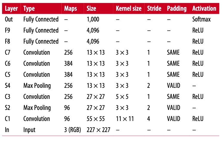
To understand the hidden layers, let us look at the table below.
So there are a total of 8 hidden layers. The real image is, i.e., input layer of size 227×227×3 is converted into a hidden layer of size 55×55×96. This is because the filter size is 11×11×96. Here 96 is the total number of kernels in the filer. According to the formula (W - F + 2×P)/S + 1 we get (227 - 11 + 2*0)/4 + 1 = 55, therefore the size of the hidden layer 1 is 55×55×96. Now the max-pooling is applied to the first hidden layer with stride = 2 and kernel size of 3×3. Note that the filter does not change while applying the max-pooling layer. So, the size of the second hidden layer will be 27×27×96.
The last three hidden layers of the AlexNet are of size 4096, 4096, 1000, respectively; these are called fully connected layers or dense layers.
Techniques used in AlexNet
To reduce overfitting, the authors used two regularization techniques: the first technique is about applying dropout regularization in the last two hidden layers, i.e., F8 and F9 layer of the AlexNet model with the dropout rate of 50%. Secondly, they performed the data augmentation on the input data, i.e., training images. Data augmentation includes changing the lighting conditions, flipping them horizontally, etc.
The competitive normalization step is immediately used after the ReLU step of layers C1 and C3, which is also called local response normalization.
The most strongly activated neurons inhibit other neurons in neighboring feature maps at the same position. This encourages different feature maps to specialize, ultimately improving generalization, pushing them apart, and forcing them to explore a wider range of features.
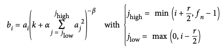
The following image shows how to apply Local Response Normalization:
ai represents the activation of that neuron after the ReLU step and before the normalization.
k, α, β, and r are hyperparameters where r is called the depth radius, and k is called bias.
fn is the number of feature maps.
The normalized output of the neuron located in feature map i is denoted by bi, at some row u and column v (note that we consider only neurons located at this row and column in this equation, so u and v are not shown).
The hyperparameters are in the AlexNet are set as follows: r = 2, α = 0.00002, β = 0.75, and k = 1. This step can be implemented using the tf.nn.local_response_normalization() function.
Implementation of AlexNet
We will be implementing the AlexNet model using tensorflow and keras libraries of python.
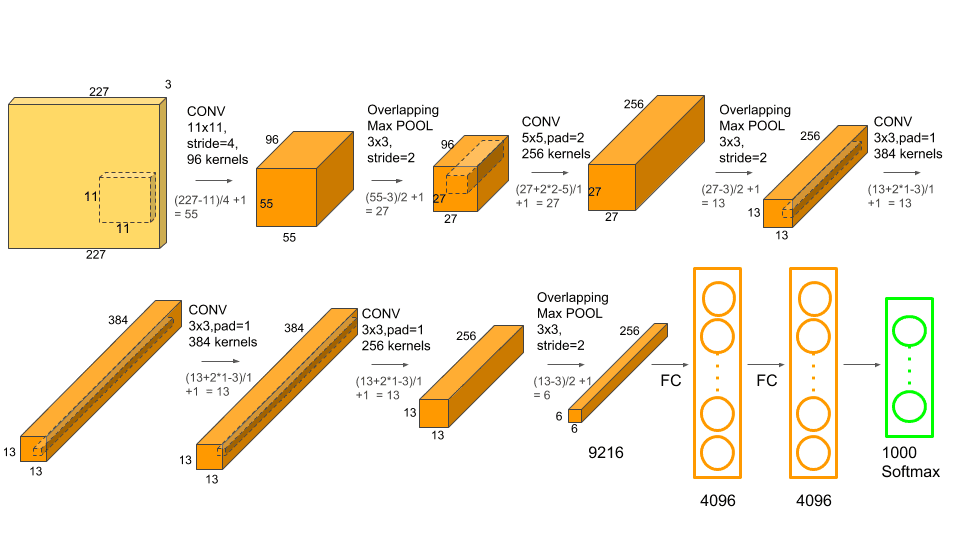
Let us see the diagram for the AlexNet and then we will implement it accordingly.
# pooling layer (S2) model.add(MaxPooling2D(strides = (2, 2),\ pool_size = (3, 3),\ padding = 'valid')) # normalizing it before passing it to the next layer model.add(BatchNormalization())
# pooling layer (S4) model.add(MaxPooling2D(strides = (2, 2),\ pool_size = (3, 3),\ padding = 'valid')) # normalizing it before passing it to the next layer model.add(BatchNormalization())
# creating third convolutional layer (C5) model.add(Conv2D(filters = 384, strides = (1, 1),\ padding = 'same',\ kernel_size = (3, 3))) # adding relu activation function model.add(Activation('relu')) # normalizing it before passing it to the next layer model.add(BatchNormalization())
# creating fourth convolutional layer (C6) model.add(Conv2D(filters = 384, strides = (1, 1),\ padding = 'same',\ kernel_size = (3, 3))) # adding relu activation function model.add(Activation('relu')) # normalizing it before passing it to the next layer model.add(BatchNormalization())
# creating fifth convolutional layer (C7) model.add(Conv2D(filters = 256, strides = (1, 1),\ padding = 'same',\ kernel_size = (3, 3))) # adding relu activation function model.add(Activation('relu')) # normalizing it before passing it to the next layer model.add(BatchNormalization())
# passing the model to dense layer model.add(Flatten())
# first dense layer model.add(Dense(4096, input_shape = (4096,))) model.add(Activation('relu')) # dropout regularization to prevent overfitting model.add(Dropout(0.5)) # normalizing it before passing it to the next layer model.add(BatchNormalization())
# second dense layer model.add(Dense(4096)) model.add(Activation('relu')) # dropout regularization to prevent overfitting model.add(Dropout(0.5)) # normalizing it before passing it to the next layer model.add(BatchNormalization())
# third dense layer model.add(Dense(1000)) model.add(Activation('relu')) # dropout regularization to prevent overfitting model.add(Dropout(0.5)) # normalizing it before passing it to the next layer model.add(BatchNormalization())
# getting the summary of the model model.summary()
Finally, use the softmax function for the last Dense layer of size 1000.
What is AlexNet used for? AlexNet is a leading architecture for any object-detection task and may have huge applications in the computer vision sector of artificial intelligence problems.
What is special about AlexNet? AlexNet can recognize off-center objects and most of its top five classes for each image are reasonable. AlexNet won the 2012 ImageNet competition with a top-5 error rate of 15.3%, compared to the second place top-5 error rate of 26.2%.
How many layers are there in AlexNet? There are total of eight layers in AlexNet, excluding the input, output, and pooling layers. Five out of eight are convolutional layers and rest three are dense layers.
Why is AlexNet so important? AlexNet was the first architecture to adopt an architecture with consecutive convolutional layers (convolutional layer 3, 4, and 5). The final fully connected layer in the network contains a softmax activation function that provides a vector that represents a probability distribution over 1000 classes.
Key Takeaways
In this article, we have discussed the following topics:
History of AlexNet
Important terminologies required to implement AlexNet
Architecture of AlexNet
Implementation of AlexNet
Hello readers, here's a perfect course that will guide you to dive deep into Machine learning.


 9+ registered

