Do you think IIT Guwahati certified course can help you in your career?
Introduction
K-Means is a popular clustering algorithm widely used in unsupervised machine learning to group data based on similarities. The Iris dataset, a classic dataset in data science, is often used to demonstrate clustering techniques due to its well-defined structure and labeled classes.
In this article, we will learn how to apply the K-Means algorithm on the Iris dataset, analyze the clustering results, and visualize the patterns identified in the data.
What is K-Means?
K-Means is an unsupervised machine learning algorithm that is used for clustering problems. Since it is an unsupervised machine learning algorithm, it uses unlabelled data to make predictions.
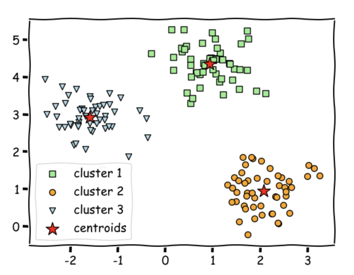
K-Means is nothing but a clustering technique that analyzes the mean distance of the unlabelled data points and then helps to cluster the same into specific groups.
In detail, K-Means divides unlabelled data points into specific clusters/groups of points. As a result, each data point belongs to only one cluster that has similar properties.
K-Means Algorithm
The various steps involved in K-Means are as follows:-
→ Choose the 'K' value where 'K' refers to the number of clusters or groups.
→ Randomly initialize 'K' centroids as each cluster will have one center. So, for example, if we have 7 clusters, we would initialize seven centroids.
→ Now, compute the euclidian distance of each current data point to all the cluster centers. Based on this, assign each data point to its nearest cluster. This is known as the 'E- Step.'
Example: Let us assume we have two points, A1(X1, Y1) and B2(X2, Y2). Then the euclidian distance between the two points would be the following:-
→ Now, update the cluster center locations by taking the mean of the data points assigned. This is known as the 'M-Step.'
→ Repeat the above two steps until convergence, i.e., until we reach a global optimum where no further optimization is possible.
We will be using the Iris Dataset and applying K-Means on the same.
The Iris Dataset helps predict the Iris flower species based on a few given properties. It consists of 5 features and one target variable.
(i) Id - ID of the flower for differentiating, numerical feature.
(ii) SepalLengthCm - sepal length of the flower, numerical feature.
(iii) SepalWidthCm - sepal width of the flower, numerical feature.
(iv) PetalLengthCm - petal length of the flower, numerical feature.
(v) PetalWidthCm - petal width of the flower, numerical feature.
(vi) Species - iris species , target variable / label.
Implementation
For simplicity, we would use the already existing sklearn library for K-Means implementation.
Importing Necessary Libraries
Firstly, we will load some basic libraries:-
(i) Numpy - for linear algebra.
(ii) Pandas - for data analysis.
(iii) Seaborn - for data visualization.
(iv) Matplotlib - for data visualisation.
(v) KMeans - for using K-Means.
(vi) LabelEncoder - for label encoding.
(vii) classification_report - for generating numerous results.
(viii) accuracy_score - for generating model accuracy.
import numpy as np import pandas as pd import seaborn as sns from matplotlib import pyplot as plt from sklearn.cluster import KMeans from sklearn.preprocessing import LabelEncoder from sklearn.metrics import classification_report from sklearn.metrics import accuracy_score
Loading Data
#loading dataset df= pd.read_csv('iris.csv')
Above, we load the data using pandas.
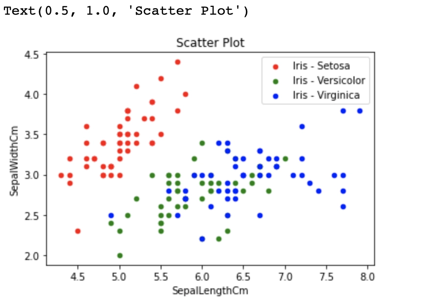
Visualization
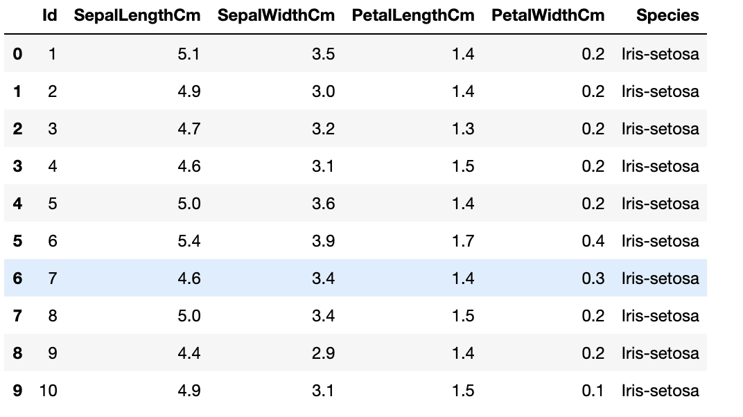
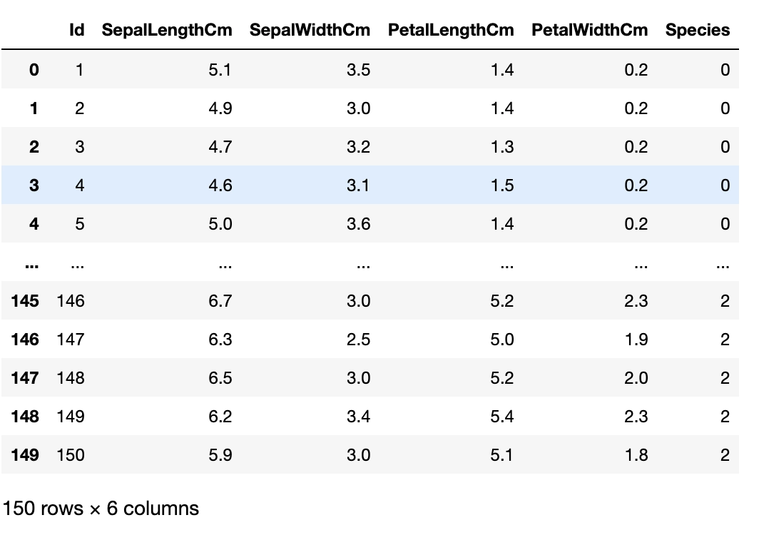
We visualize the dataset by printing the first ten rows of the data frame. We use the head() function for the same.
#visualizing dataset df.head(n=10)
Output
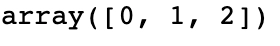
#finding different class labels np.unique(df['Species'])
Output
We notice that there are three different classes present in the dataset.
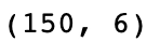
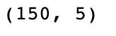
df.shape
Output
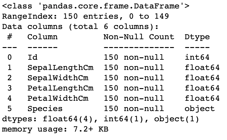
We observe that our dataset consists of 150 rows and six columns.
df.info()
Output
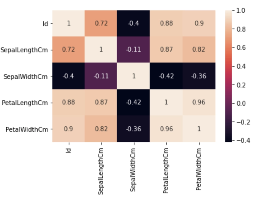
#finding correlation of features correl=df.corr() sns.heatmap(correl,annot=True)
Output
From the above, we observe that bigger values are represented with light color. This observation will always be the same for the heatmap. Dark values will always be less than light-colored values.
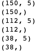
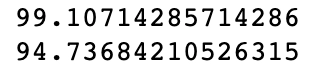
We notice that we get good results on both training and testing sets. The training set gives us a score of 99.10, whereas the testing set gives us a score of 94.73.
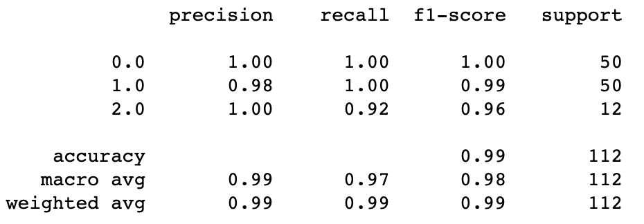
Finally, we will generate a classification report for in-depth analysis.
#classification report for training set print(classification_report(train_y, train_labels))
Output
Frequently Asked Questions
What is the advantage as well as disadvantage of KMeans?
An advantage of KMeans is that it is computationally very fast. A disadvantage of the same is that it does not work too well with clusters of different sizes.
What is the importance of clustering in ML?
Clustering helps identify and group similar data points in larger datasets without concern for the specific outcome.
What does the ‘K’ in K-Means stand for?
K’ refers to the number of clusters in K-means.
Conclusion
Congratulations on making it this far. This blog discussed a fundamental overview of KMeans along with the Iris Dataset!!
We learned about Data Loading, Data Visualisation, Data Preprocessing, and Training. We learned how to visualize data then, based on this EDA, took significant decisions concerning preprocessing, made our model training ready, and finally generated the results for it.
If you are preparing for the upcoming Campus Placements, don’t worry. Coding Ninjas has your back. Visit this link for a carefully crafted and designed course on-campus placements and interview preparation.


 8+ registered

