Applying Logistic Regression on Iris dataset

Introduction

There are several machine learning models present today. Different types of models, like different people, have their specialties and fields where they excel more than others. Here in this article, we are going to employ the services of the Logistic Regression Model on the Iris Dataset to predict the species of the flower. 

Logistic Regression is used to predict a dependent variable, given a set of independent variables, such that the dependent variable is categorical.

The Logistic function is an S-shaped curve that can take any real-valued number and map it into a value between 0 and 1. 

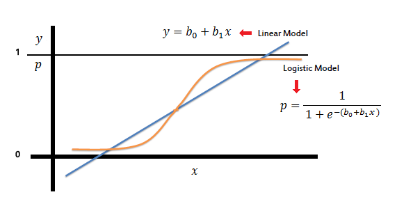
Source: saedsayed.com

Sigmoid function: 11+e-x , x is the independent variable.

Implementation

Let's import some essential modules. 

import pandas as pd
# used to read the data set
import numpy as np
# used to do some operations with the arrays
import os
# used handle some files
import matplotlib.pyplot as plt
# used to visualize the data using graphs
import seaborn as sns
# plotting the chart in a single line

 

Let's load the dataset (see Pandas).

df = pd.read_csv("Iris.csv")

 

The data set will be read and stored in the data frame format.

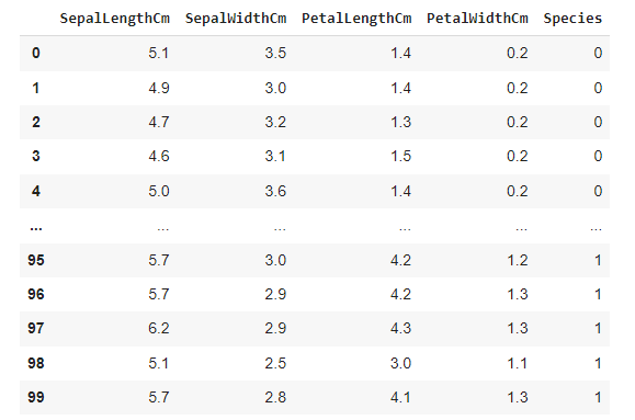
Let’s display the first five rows of the data set.

 

df.head(5)

 

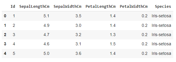
We have four features, SepalLength, SepalWidth, PetalLength, and PetalWidth. The last feature, 'Species,' is the target feature that will be predicted.

Feature 'Id' is a definite feature that does not affect the target feature. So let's drop that feature.

 

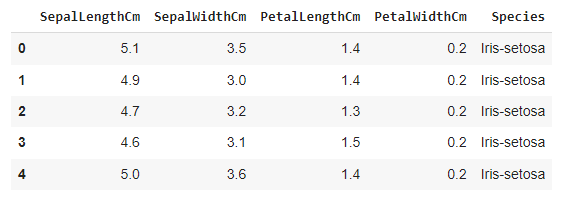
df = df.drop(columns = ['Id'])
df.head(5)

 

 

Let’s have the information about the data type of the data set.

 

df.info()

 

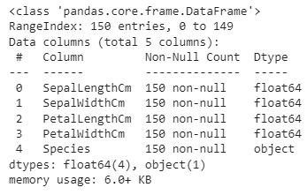
SepalLength, SepalWidth, PetalLength, and PetalWidth have float data types. 'Species' has an object data type. Let's check the number of samples of each class in Species.

 

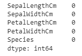
df['Species'].value_counts()

 

 

In each class, we have fifty samples.

While training the model, we must remove all the null values with other deals like mean, median, mode, etc. To check whether the data set contains the null values, We write.

 

df.isnull().sum()

 

It will display the number of null values in each column.

 

 

There are no null or nan values in the datasets.

Now, We will visualize the data in the form of graphs. First, let's display some basic charts. For each column, let us create a histogram.

 

df['SepalLengthCm'].hist()
df['SepalWidthCm'].hist()

 

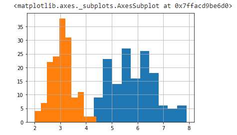
          Blue - SepalLenth

          Orange- SepalWidth

 

df['PetalLengthCm'].hist()
df['PetalWidthCm'].hist()

 

 

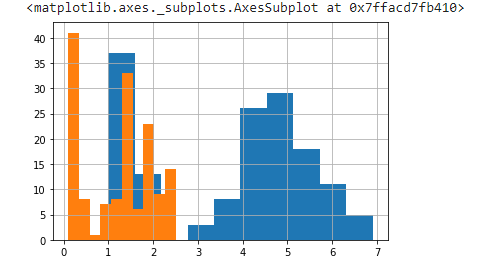
        Blue- PetalLength

        Orange- PetalWidth

 

We can observe that the histogram plot of all the features follows the normal distribution. 

PDF of the normal distribution with mean μ and variance σ2 is given by:

 

 

 

If the size of the data set is large enough, the normal distribution is a good approximation.

A correlation matrix shows the correlation between the two variables. The value is in the range of -1 to +1. If two variables have a correlation much nearer to +1 or -1, we can neglect one variable.

So we are going to construct the matrix from the input attributes.

If you want to learn more about covariance and correlation check out Covariance and Correlation

 

df.corr()

 

 

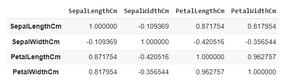
Here, the correlation coefficient between PetalLength and PetalWidth is 0.962757, which is much closer to 1, so we can remove any of the two variables. A correlation coefficient is a convenient tool when we have lots of features, and we can neglect multiple features by observing the correlation coefficient matrix. 

 

In Machine learning, we usually deal with the dataset which contains multiple labels in columns. These labels can be in the form of words or numbers. Label Encoding refers to converting the labels into the numeric form into the machine-readable form.

The output class is in the categorical form in this data set, and we need to convert it into the numeric format. So We will use Label Encoder.

from sklearn.preprocessing import LabelEncoder
le = LabelEncoder()
df['Species'] = le.fit_transform(df['Species'])
df.head(100)

 

 

After preprocessing all the data sets, we need to train and test our model. So, let's import the model.

 

from sklearn.model_selection import train_test_split

 

We need to separate the classes for input and output attributes. Let's drop the columns ‘Species’ and store the remaining input attributes to the variable X. The output attribute, i.e., ‘Species,’ is taken in the variable Y.

 

X = df.drop(columns = ['Species'])
Y = df['Species']
X_train, X_test, Y_train, Y_test = train_test_split(X, Y, test_size = 0.25)

 

Now let's import a basic classification model called logistic Regression from SKlearn.

 

from sklearn.linear_model import LogisticRegression
model = LogisticRegression()

 

Now, let's train the model.

 

model.fit(X_train, Y_train)

 

Let's print the metric to get the performance.

 

print("Accuracy: ", model.score(X_test, Y_test) * 100)

 

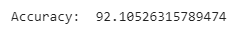
We are getting an accuracy of 92%, which is very decent. The accuracy increases with the increase in the number of data points.
Check out this problem - Largest Rectangle in Histogram