


Introduction
Cryptography is an important part of the digital world today. It is how we protect the vast amounts of digital information that exist on thousands of servers worldwide. To ensure that cryptography remains strong and cannot be hacked, we ourselves need to study methods to break cryptographic algorithms. This helps us learn about weaknesses in our ciphers and how to remove those weaknesses.

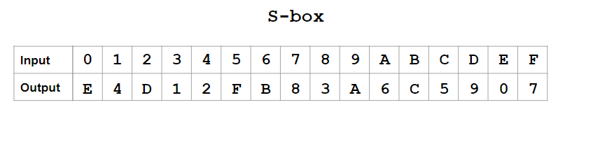
S-boxes are a common part of many cryptographic ciphers. There are many ways that have been tried to break them and find flaws. Linear Cryptanalysis is one of them. To perform linear cryptanalysis, we first need to perform a Linear Approximation of the S-box. Let us see what it is and how we can do it.
Basic Concepts
Cryptography involves a lot of probability. To properly understand the linear approximation of S-boxes, we will need some basic concepts of probability and random variables.
To learn about S-boxes, you can read our article SPN in Cryptography. For Random Variables, you can read the articles Introduction to Random Variables and Random Variables.
Linear Approximation of S-boxes is important because non-linear S-boxes are considered cryptographically secure. S-boxes, and even other cryptographical tools, that have linear properties are considered vulnerable to many attacks.
Linear properties are those that we can easily estimate and predict using probabilistic analysis. They allow us to predict which plaintext will result in which ciphertext, or vice versa. This is because S-boxes with linear properties tend to have bias. We will look at all of this in detail in the upcoming sections.
Notations and Basic Equations
We will be using the following notation throughout the article.
Pr[X=x] represents the probability that the random variable X takes the value x.
Pr[x] is used to represent the same thing, when X is understood.
Pr[x,y] represents the probability that X=x and Y=y.
Pr[x|y] represents the probability that X=x, given that Y=y.
The following results can be concluded from the above definition.
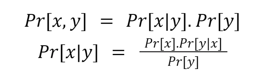
The second equation is the famous Bayes Theorem.
XOR and Bias
Suppose X1, X2,.... are independent random variables that can take values 0 and 1.
Let
pi = Pr[Xi=0]
Then,
1-pi = Pr[Xi=1]
For Xi and Xj, the independence of Xi and Xj implies that:
Pr[Xi=0,Xj=0] = pipj
Pr[Xi=0,Xj=1] = pi(1-pj)
Pr[Xi=1,Xj=0] =(1- pi )pj
Pr[Xi=1,Xj=1] = (1-pi)(1-pj )
Let's consider a new random variable Y = Xi ⊕ Xj.
It's easy to see that
Pr[Y=0]=Pr[Xi ⊕ Xj=0] = pipj+ (1-pi)(1-pj )
Pr[Y=1]=Pr[Xi ⊕ Xj=1] = pi(1-pj)+ (1-pi)pj
This is because ⊕ gives output 1 when both inputs are different, otherwise the output is 0.
Bias is a commonly used term in probability theory and is used in probability distribution of random variables. The bias of the random variable Xi is defined as:
∊i = pi - ½
Piling-up Lemma
Let i1,i2,i3,....ik denote the bias of the random variable Xi1 ⊕ Xi2 ⊕ Xi3 ⊕ …..⊕ Xik, then:
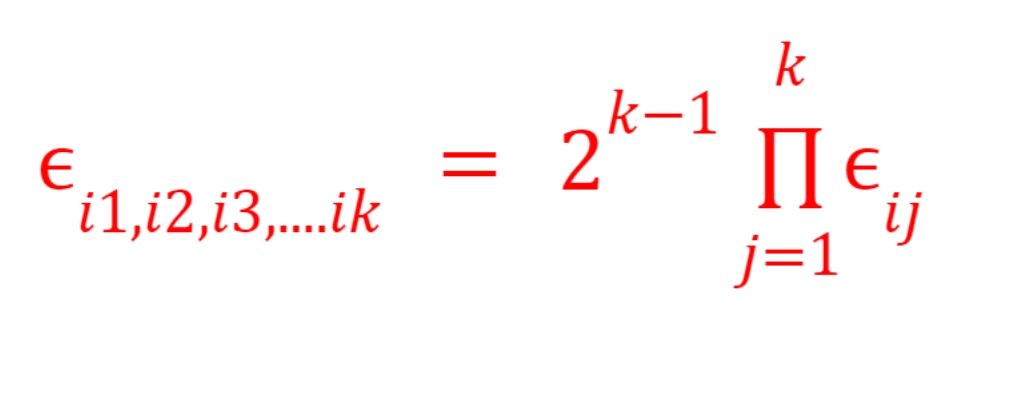
For example:
The bias of X1 ⊕ X3 ⊕ X6 will be
∊1,3,6 = 22 ∊1.∊3.∊6
With these basic concepts, we can start doing the linear approximation of S-boxes. To learn more about Piling-up lemma, you can visit our article on Linear Cryptanalysis.


 9+ registered

