Table of contents
1.
Introduction
2.
Introduction to Time Series Forecasting
3.
Introduction to ARIMA
4.
Architecture of ARIMA model
5.
Implementing analysis with ARIMA Model
6.
Frequently Asked Questions
6.1.
What is the difference between time series analysis and time series forecasting?
6.2.
Is it important for a Time Series to be Stationary in the ARIMA model?
6.3.
What is SARIMA?
7.
Conclusion
Last Updated: Mar 27, 2024
Easy

ARIMA Model for Time Series Analysis

Author Komal
0 upvote
Career growth poll
Do you think IIT Guwahati certified course can help you in your career?

Introduction

Welcome Ninjas! Have there been times when you were watching a cricket match and guessed that this team might win based on its performance in previous matches? This is what Time Series Forecasting is all about, Predicting the future value based on the historical data we have.

 ARIMA Model for Time Series Analysis

In this blog, we will be learning about time series forecasting and a widely used approach, ARIMA, for the same. The blog will then follow the implementation and analysis of the ARIMA model.

Introduction to Time Series Forecasting

Time series forecasting refers to predicting future data based on historical data. Historical data is first analyzed. Then, the patterns(trends, cyclic patterns, etc.) are found and used in further prediction. In simpler words, we estimate the future value based on what has already happened.

Prediction problems involving a time component require time series forecasting. It provides a data-driven approach to effective and efficient planning.

Applications

Time Series is used in the study of various fields, some of them are mentioned below:

  • Astronomy
  • Business planning
  • Control engineering
  • Earthquake prediction
  • Econometrics
  • Mathematical finance
  • Pattern recognition
  • Resources allocation
  • Signal processing
  • Statistics
  • Weather forecasting

Introduction to ARIMA

Now, What is the ARIMA model? ARIMA model is used as an approach for time series forecasting. The name ARIMA can be split into three parts:-
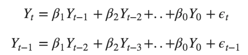
AutoRegression (AR)

AR tends to indicate the regression of a variable against itself, i.e., the output of a model is linearly dependent on its previous value. It also represents a type of random access. 

AR

Moving Average (MA)

In a MA model, the output is linearly dependent on past forecast errors. 

MA

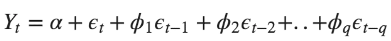
Where the error terms are based on errors from the equations given below:

MA

Moreover, when we combine the AR and MR terms, we get the equation:

AR+MA

Integrated (I)

integrated refers to removing the trend and seasonal components. It is done to form stationary time series data.


Architecture of ARIMA model

Before implementing the ARIMA model, we must note the three components of the model- p, q & d.

We identify the ARIMA model by three terms:

p- refers to the order of the AR term

q- refers to the order of the MA term

d- refers to the number of differencing to make time series stationary.

Implementing analysis with ARIMA Model

Let's now build the ARIMA model for time series analysis. We will be going through several steps to achieve the same.

Implementing ARIMA in R

First, we read the dataset. Note that in this blog, we will be using the dataset - ‘WWWusage.txt’ available online.

usage=scan('C:/Users/komal/Desktop/wwwusage.txt', skip=1)

Then, we plot the dataset.

plot(1:100, usage, xlim = c(0, 100), ylim=c(80, 250))

To connect the points,

lines(1:100, df, type="l")
Plot the dataset

Interpretation of sample ACF and PACF plot

Autocorrelation coefficient function(ACF) refers to how the data points are related to the preceding data points.points.

Partial autocorrelation coefficient function(PACF) specifies  specifies  the dependence structure of a stationary process.

acf(usage, lag.max=100)
acf
pacf(usage, lag.max=100)
pacf

We conclude that the data is not stationary.

Now, we take first order differencing,

z = diff(usage, 1, 1)
plot(1:99, z, xlim = c(0, 100), ylim=c(-15, 15))
lines(1:99, z, type="l" )
plot
acf(z, lag.max=100)
pacf(z, lag.max=100)


acf


pacf

Take second order differencing,

z = diff(usage, 1, 2)
plot(1:98, z, xlim = c(0, 120), ylim=c(-15, 15))
lines(1:98, z, type="l" )
plot
acf(z, lag.max=100)
pacf(z, lag.max=100)


acf


pacf

Now, the ACF decay very fast, so the data is stationary

Now, before going further, we should know what AIC is. AIC is the Akaike Information Criteria. It is a widely used measure of a statistical model. It helps in quantifying the goodness of a statistical fit and the simplicity of a model in a single statistic.

Model-1 ARIMA

ft = arima(usage, order = c(0,2,2))
tsdiag(ft)                             
Model1


summary

The AIC criterion value for Model 1 ARIMA(0,2,2) = 517.211

Model-2 ARIMA

ft2 = arima(usage, order = c(2,2,0))
tsdiag(ft2)
Model-2 ARIMA
Model-2 ARIMA

The AIC criterion value for Model 2 ARIMA(2,2,0) = 511.46

Model-3 ARIMA

library(forecast)
ft3 = auto.arima(usage)
tsdiag(ft3)


model3
summary

The AIC value for model 3 ARIMA(1,1,1) = 514.55

 It's known that lower the AIC criterion value, the better the model. Observing the AIC values of the models, we choose the Model 2 ARIMA (2,2,0) as the final fitted model  for wwwusage data as it gives the lowest AIC (511.46). 

Frequently Asked Questions

What is the difference between time series analysis and time series forecasting?

In time series analysis, we understand and analyze the dataset. In forecasting, we predict based on the analysis already made.

Is it important for a Time Series to be Stationary in the ARIMA model?

Yes, Stationarity is very important because a model describing the data might vary in accuracy at different time points in its absence.

What is SARIMA?

SARIMA refers to Seasonal-ARIMA and the name is justified as it includes seasonality contribution. The importance of seasonality is evident.

Conclusion

We hope this blog helped you understand the fundamental concepts of Time Series Analysis along with the ARIMA model and it's implementation

If you found this blog interesting and insightful, you can refer to similar blogs on Coding Ninjas Studio.

Refer to the Basics of C++ with Data StructureDBMS, and Operating System by Coding Ninjas, and keep practicing on our platform Coding Ninjas Studio. You can check out the mock test series on code studio.

You can also refer to our Guided Path on Coding Ninjas Studio to upskill yourself in domains like Data Structures and AlgorithmsCompetitive ProgrammingAptitude, and many more! Refer to the interview bundle if you want to prepare for placement interviews. Check out interview experiences to understand various companies' interview questions.

Give your career an edge over others by considering our premium courses!

Happy Learning!

Thankyou image
Live masterclass