Working of Bahdanau Attention Model
Only a few source positions are focused on in Bahdanau or Local attention. Global attention is computationally expensive because it focuses on all source side words for all target words. To compensate for this shortcoming, local attention chooses to focus on only a tiny subset of the encoder's hidden states per target word.
Local attention locates an alignment point, calculates the attention weight in the left and right windows where its location is found, and then weights the context vector. The main benefit of local attention is that it lowers the cost of calculating the attention mechanism.
The local attention is used in the computation to forecast the position of the source language end to be aligned at the present decoding using a prediction function and then travel through the context window, only considering the words within the window.
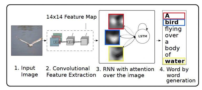
Now, let us implement a model that will help understand the attention mechanism in image captioning.
Image Captioning
I will be implementing the model using the Flickr 8k dataset. The link for the dataset is given here. The dataset has 8000 different images and each image has five different captions.
Importing libraries
import numpy as np
import pandas as pd
import string
from numpy import array
from PIL import Image
from pickle import load
import pickle
import matplotlib.pyplot as plt
from collections import Counter
import sys, time, os, warnings
warnings.filterwarnings("ignore")
from tqdm import tqdm
import re
import keras
from nltk.translate.bleu_score import sentence_bleu
import tensorflow as tf
from keras.preprocessing.sequence import pad_sequences
from tensorflow.keras.utils import to_categorical, plot_model
from keras.models import Model
from keras.layers import Input, Dense, BatchNormalization, LSTM, Embedding, Dropout
from keras.layers.merge import add
from keras.callbacks import ModelCheckpoint
from keras.preprocessing.text import Tokenizer
from keras.preprocessing.image import load_img, img_to_array
from keras.applications.vgg16 import VGG16, preprocess_input
from sklearn.model_selection import train_test_split
from sklearn.utils import shuffle

You can also try this code with Online Python Compiler
Loading Data
I am using google colab for training the model, and I am loading the dataset directly from google drive.
image_path = "/content/drive/MyDrive/Datasets/archive/Images"
dir_Flickr_text = "/content/drive/MyDrive/Datasets/archive/captions.txt"
jpgs = os.listdir(image_path)

print("Total Images in Dataset = {}".format(len(jpgs)))
You can also try this code with Online Python Compiler
Total Images in Dataset = 8101
You can also try this code with Online Python Compiler
Data Preprocessing
Firstly, we will make a dataframe of image names associated with its captions.
file = open(dir_Flickr_text,'r')
text = file.read()
file.close()
datatxt = []
i = 0
for line in text.split('\n'):
try:
col = line.split('\t')
col = col[0].split(',')
w = col[0].split("#")
if i == 0:
i+=1
continue
i+=1
datatxt.append(w + [col[1].lower()])
except:
continue
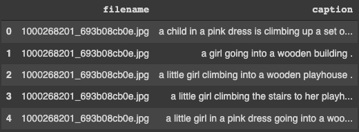
data = pd.DataFrame(datatxt,columns=["filename","caption"])
data = data[data.filename != '2258277193_586949ec62.jpg.1']
uni_filenames = np.unique(data.filename.values)
data.head()
You can also try this code with Online Python Compiler
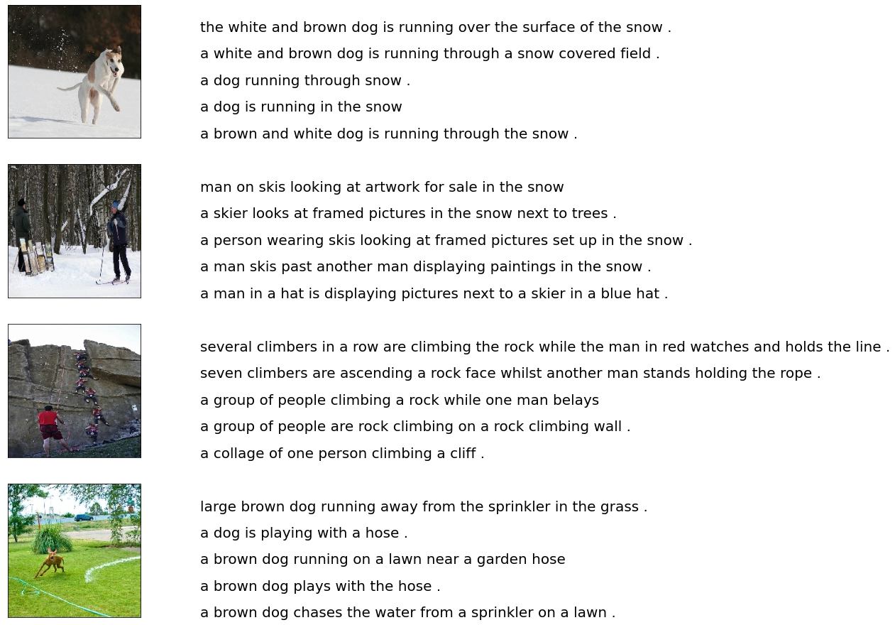
Next, we will visualize some images with their respective 5 captions.
npc = 5
npx = 224
t_sz = (npx,npx,3)
count = 1

Figure = plt.figure(figsize=(10,20))
for i in uni_filenames[10:14]:
  fname = image_path + '/' + i
  captions = list(data["caption"].loc[data["filename"]==i].values)
  image_load = load_img(fname, t_sz=t_sz)
  axs = Figure.add_subplot(npc,2,count,xticks=[],yticks=[])
  axs.imshow(image_load)
  count += 1

  axs = Figure.add_subplot(npc,2,count)
  plt.axis('off')
  axs.plot()
  axs.set_xlim(0,1)
  axs.set_ylim(0,len(captions))
  for i, caption in enumerate(captions):
      axs.text(0,i,caption,fontsize=20)
  count += 1
plt.show()
You can also try this code with Online Python Compiler
Let us see the size of the current vocabulary.
vocabulary = []
for txt in data.caption.values:
  vocabulary.extend(txt.split())
print('Vocabulary is of size: %d' % len(set(vocabulary)))
You can also try this code with Online Python Compiler
Vocabulary is of Size: 8182
You can also try this code with Online Python Compiler
Now we will do some text cleaning on the caption, i.e., removing punctuation, removing single characters, removing numerical values.
def punctuation_removal(text_original):
  tnp = text_original.translate(string.punctuation)
  return(tnp)

def single_character_removal(text):
  tlmt1 = ""
  for word in text.split():
      if len(word) > 1:
          tlmt1 += " " + word
  return(tlmt1)

def number_removal(text):
  tnn = ""
  for word in text.split():
      isalpha = word.isalpha()
      if isalpha:
          tnn += " " + word
  return(tnn)

def text_cleaner(text_original):
  text = punctuation_removal(text_original)
  text = single_character_removal(text)
  text = number_removal(text)
  return(text)

for i, caption in enumerate(data.caption.values):
  nc = text_cleaner(caption)
  data["caption"].iloc[i] = nc
You can also try this code with Online Python Compiler
Let’s check the size of the dataset after cleaning the dataset.
clean = []
for txt in data.caption.values:
  clean.extend(txt.split())
print('Clean Vocabulary Size: %d' % len(set(clean)))
You can also try this code with Online Python Compiler
Clean Vocabulary Size: 8182
You can also try this code with Online Python Compiler
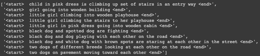
Next, we save all of the descriptions and picture paths in two separate lists so that we can use the path set to load all of the images at once. We also add '<start >' and '<end >' tags to each caption so that the model can understand where each caption begins and ends.
PATH = "/content/drive/MyDrive/Datasets/archive/Images/"
total_captions = []
for cp  in data["caption"].astype(str):
  cp = '<start> ' + cp+ ' <end>'
  total_captions.append(cp)

total_captions[:10]
You can also try this code with Online Python Compiler
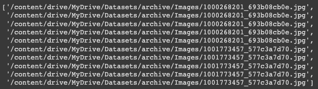
img_vectors = []
for annotations in data["filename"]:
  image_paths = PATH + annotations
  img_vectors.append(image_paths)

img_vectors[:10]
You can also try this code with Online Python Compiler
Now we will see the size of captions and image path vectors.
print(f"len(img_vectors) : {len(img_vectors)}")
print(f"len(total_captions) : {len(total_captions)}")
You can also try this code with Online Python Compiler
len(all_img_name_vector) : 40455
len(all_captions) : 40455
You can also try this code with Online Python Compiler
We'll just take 40000 of each so we can properly set batch size, i.e. 625 batches if batch size=64. To do this, we create a function that restricts the dataset to 40000 photos and descriptions.
def data_limiter(nums,tc,imv):
training_captions, image_vector = shuffle(tc,imv,random_state=1)
training_captions = training_captions[:nums]
image_vector = image_vector[:nums]
return training_captions,image_vector

train_captions,img_name_vector = data_limiter(40000,total_captions,img_vectors)
You can also try this code with Online Python Compiler
Model Making
Let's use VGG16 to define the image feature, extraction model. It's important to note that we don't need to classify the images here; all we need to do is extract an image vector. As a result, the softmax layer is removed from the model. Before feeding the photos into the model, we must all preprocess them to the same size, 224×224.
def load_image(path):
image = tf.io.read_file(path)
image = tf.image.decode_jpeg(image, channels=3)
image = tf.image.resize(image, (224, 224))
image = preprocess_input(image)
return image, path
image_model = tf.keras.applications.VGG16(include_top=False, weights='imagenet')
new_input = image_model.input
hidden_layer = image_model.layers[-1].output
image_features_extract_model = tf.keras.Model(new_input, hidden_layer)
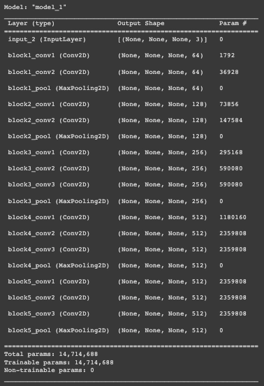
image_features_extract_model.summary()
You can also try this code with Online Python Compiler
Next, let’s Map each image name to the function to load the image:
encode_train = sorted(set(img_name_vector))
image_dataset = tf.data.Dataset.from_tensor_slices(encode_train)
image_dataset = image_dataset.map(load_image, num_parallel_calls=tf.data.experimental.AUTOTUNE).batch(64)
You can also try this code with Online Python Compiler
We extract the features and save them in the appropriate .npy files, after which we pass them through the encoder. NPY files include all of the data needed to recreate an array on any machine, including dtype and shape data.
%%time
for img, path in tqdm(image_dataset):
batch_features = image_features_extract_model(img)
batch_features = tf.reshape(batch_features,
                            (batch_features.shape[0], -1, batch_features.shape[3]))

for bf, p in zip(batch_features, path):
  path_of_feature = p.numpy().decode("utf-8")
  np.save(path_of_feature, bf.numpy())
You can also try this code with Online Python Compiler
Now, we will tokenize the captions and will build a vocabulary of 5000 unique words from the data. The words that are not in the vocabulary will be marked as <unk>.
topk = 5000
tkn = tf.keras.preprocessing.text.Tokenizer(num_words=topk,
                                                oov_token="<unk>",
                                                filters='!"#$%&()*+.,-/:;=?@[\]^_`{|}~ ')

tkn.fit_on_texts(train_captions)
train_seqs = tkn.texts_to_sequences(train_captions)
tkn.word_index['<pad>'] = 0
tkn.index_word[0] = '<pad>'

train_seqs = tkn.texts_to_sequences(train_captions)
cap_vector = tf.keras.preprocessing.sequence.pad_sequences(train_seqs, padding='post')
You can also try this code with Online Python Compiler
train_captions[:3]
You can also try this code with Online Python Compiler

train_seqs[:3]
You can also try this code with Online Python Compiler
Let us see the maximum and minimum length of the captions.
def max_sz(tensor):
  return max(len(t) for t in tensor)
mx_l = max_sz(train_seqs)

def min_sz(tensor):
  return min(len(t) for t in tensor)
min_l = min_sz(train_seqs)

print('Max Length of any caption : Min Length of any caption = '+ str(mx_l) +" : "+str(min_length)min_l)
You can also try this code with Online Python Compiler
Max Length of any caption : Min Length of any caption = 31 : 2
You can also try this code with Online Python Compiler
Training Model
Now we will split the data using train_test_split.
img_name_train, img_name_val, cap_train, cap_val = train_test_split(img_name_vector,cap_vector, test_size=0.2, random_state=0)
You can also try this code with Online Python Compiler
Defining the training parameters
BATCH_SIZE = 64
BUFFER_SIZE = 1000
embedding_dim = 256
units = 512
vocab_size = len(tokenizer.word_index) + 1
num_steps = len(img_name_train) // BATCH_SIZE
features_shape = 512
attention_features_shape = 49
You can also try this code with Online Python Compiler
Next, let’s create a tf.data dataset to use for training our model.
def map_function(img_name, cap):
tensor_img = np.load(img_name.decode('utf-8')+'.npy')
return tensor_img, cap
dataset = tf.data.Dataset.from_tensor_slices((img_name_train, cap_train))

dataset = dataset.map(lambda item1, item2: tf.numpy_function(
      map_function, [item1, item2], [tf.float32, tf.int32]),
        num_parallel_calls=tf.data.experimental.AUTOTUNE)

dataset = dataset.shuffle(BUFFER_SIZE).batch(BATCH_SIZE)
dataset = dataset.prefetch(buffer_size=tf.data.experimental.AUTOTUNE)
You can also try this code with Online Python Compiler
Let us define the encoder-decoder model with attention.
class VGG16_Encoder(tf.keras.Model):
  def __init__(self, embedding_dim):
      super(VGG16_Encoder, self).__init__()
      self.fc = tf.keras.layers.Dense(embedding_dim)
      self.dropout = tf.keras.layers.Dropout(0.5, noise_shape=None, seed=None)

  def call(self, x):
      x = self.fc(x)
      x = tf.nn.relu(x)
      return x
You can also try this code with Online Python Compiler
Defining RNN
def rnn_type(units):
  if tf.test.is_gpu_available():
      return tf.compat.v1.keras.layers.CuDNNLSTM(units,
                                      return_state=True,
                                      return_sequences=True,
                                      recurrent_initializer='glorot_uniform')
  else:
      return tf.keras.layers.GRU(units,
                                return_state=True,
                                return_sequences=True,
                                recurrent_activation='sigmoid',
                                recurrent_initializer='glorot_uniform')
You can also try this code with Online Python Compiler
Defining RNN Decoder with Bahdanau Attention.
class Rnn_Local_Decoder(tf.keras.Model):
def __init__(self, embedding_dim, units, vocab_size):
  super(Rnn_Local_Decoder, self).__init__()
  self.units = units
  self.embedding = tf.keras.layers.Embedding(vocab_size, embedding_dim)
  self.gru = tf.keras.layers.GRU(self.units,
                                return_sequences=True,
                                return_state=True,
                                recurrent_initializer='glorot_uniform')
  self.fc1 = tf.keras.layers.Dense(self.units)

  self.dropout = tf.keras.layers.Dropout(0.5, noise_shape=None, seed=None)
  self.batchnormalization = tf.keras.layers.BatchNormalization(axis=-1, momentum=0.99, epsilon=0.001, center=True, scale=True, beta_initializer='zeros', gamma_initializer='ones', moving_mean_initializer='zeros', moving_variance_initializer='ones', beta_regularizer=None, gamma_regularizer=None, beta_constraint=None, gamma_constraint=None)

  self.fc2 = tf.keras.layers.Dense(vocab_size)

  # Attention Mechanism
  self.Uattn = tf.keras.layers.Dense(units)
  self.Wattn = tf.keras.layers.Dense(units)
  self.Vattn = tf.keras.layers.Dense(1)

def call(self, x, features, hidden):
  hidden_with_time_axis = tf.expand_dims(hidden, 1)
  score = self.Vattn(tf.nn.tanh(self.Uattn(features) + self.Wattn(hidden_with_time_axis)))
  attention_weights = tf.nn.softmax(score, axis=1)
  context_vector = attention_weights * features
  context_vector = tf.reduce_sum(context_vector, axis=1)
  x = self.embedding(x)
  x = tf.concat([tf.expand_dims(context_vector, 1), x], axis=-1)
  output, state = self.gru(x)
  x = self.fc1(output)
  x = tf.reshape(x, (-1, x.shape[2]))
  x= self.dropout(x)
  x= self.batchnormalization(x)
  x = self.fc2(x)
  return x, state, attention_weights

def reset_state(self, batch_size):
  return tf.zeros((batch_size, self.units))

encoder = VGG16_Encoder(embedding_dim)
decoder = Rnn_Local_Decoder(embedding_dim, units, vocab_size)
You can also try this code with Online Python Compiler
Defining optimizer and loss function.
optimizer = tf.keras.optimizers.Adam()
loss_object = tf.keras.losses.SparseCategoricalCrossentropy(
  from_logits=True, reduction='none')

def loss_function(real, pred):
mask = tf.math.logical_not(tf.math.equal(real, 0))
loss_ = loss_object(real, pred)
mask = tf.cast(mask, dtype=loss_.dtype)
loss_ *= mask

return tf.reduce_mean(loss_)
You can also try this code with Online Python Compiler
Training Model
Let's go on to define the training stage. We use a technique known as Teacher Forcing, which involves passing the target word to the decoder as the next input. This strategy aids in fast learning the correct sequence or statistical features for the sequence.
loss_plot = []

@tf.function
def train_step(img_tensor, target):
loss = 0
hidden = decoder.reset_state(batch_size=target.shape[0])
dec_input = tf.expand_dims([tokenizer.word_index['<start>']] * BATCH_SIZE, 1)

with tf.GradientTape() as tape:
    features = encoder(img_tensor)
    for i in range(1, target.shape[1]):
        predictions, hidden, _ = decoder(dec_input, features, hidden)
        loss += loss_function(target[:, i], predictions)
        dec_input = tf.expand_dims(target[:, i], 1)

total_loss = (loss / int(target.shape[1]))
trainable_variables = encoder.trainable_variables + decoder.trainable_variables
gradients = tape.gradient(loss, trainable_variables)
optimizer.apply_gradients(zip(gradients, trainable_variables))

return loss, total_loss
You can also try this code with Online Python Compiler
Training the model.
EPOCHS = 20
for epoch in range(0, EPOCHS):
  start = time.time()
  total_loss = 0
  for (batch, (img_tensor, target)) in enumerate(dataset):
      batch_loss, t_loss = train_step(img_tensor, target)
      total_loss += t_loss
      if batch % 100 == 0:
          print ('Epoch {} Batch {} Loss {:.4f}'.format(
            epoch + 1, batch, batch_loss.numpy() / int(target.shape[1])))
  loss_plot.append(total_loss / num_steps)
  print ('Epoch {} Loss {:.6f}'.format(epoch + 1
                                      total_loss/num_steps))
  print ('Time taken for 1 epoch {} sec\n'.format(time.time() - start))
You can also try this code with Online Python Compiler
Greedy Search and BLEU Evaluation
Defining a greedy method of defining captions
def evaluate(image):
  ap = np.zeros((max_length, attention_features_shape))
  hdn = decoder.reset_state(batch_size=1)
  ti = tf.expand_dims(load_image(image)[0], 0)
  itv = image_features_extract_model(ti)
  itv = tf.reshape(itv, (itv.shape[0], -1, itv.shape[3]))
  ftrs = encoder(itv)
  dec_input = tf.expand_dims([tokenizer.word_index['<start>']], 0)
  result = []
  for i in range(max_length):
      predictions, hdn, attention_weights = decoder(dec_input, ftrs, hdn)
      ap[i] = tf.reshape(attention_weights, (-1, )).numpy()
      predicted_id = tf.argmax(predictions[0]).numpy()
      result.append(tokenizer.index_word[predicted_id])

      if tokenizer.index_word[predicted_id] == '<end>':
          return result, ap

      dec_input = tf.expand_dims([predicted_id], 0)
  ap = ap[:len(result), :]

  return result, ap
You can also try this code with Online Python Compiler
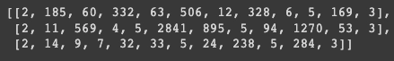
Plotting attention maps for each generated word.
def plot_attention(image, result, attention_plot):
  ti = np.array(Image.open(image))
  f = plt.figure(figsize=(10, 10))
  lr = len(result)
  for l in range(lr):
      temp_att = np.resize(attention_plot[l], (8, 8))
      ax = f.add_subplot(lr//2, lr//2, l+1)
      ax.set_title(result[l])
      img = ax.imshow(ti)
      ax.imshow(temp_att, cmap='gray', alpha=0.6, extent=img.get_extent())

  plt.tight_layout()
  plt.show()
You can also try this code with Online Python Compiler
Constructing captions for the images.
r = np.random.randint(0, len(img_name_val))
photo = img_name_val[r]
start = time.time()
real_caption = ' '.join([tokenizer.index_word[i] for i in cap_val[r] if i not in [0]])
result, attention_plot = evaluate(photo)
first = real_caption.split(' ', 1)[1]
real_caption = first.rsplit(' ', 1)[0]
for i in result:
if i=="<unk>":
result.remove(i)
#remove <end> from result
result_join = ' '.join(result)
result_final = result_join.rsplit(' ', 1)[0]
real_appn = []
real_appn.append(real_caption.split())
reference = real_appn
candidate = result_final
print ('Real Caption:', real_caption)
print ('Prediction Caption:', result_final)
plot_attention(photo, result, attention_plot)
print(f"time took to Predict: {round(time.time()-start)} sec")
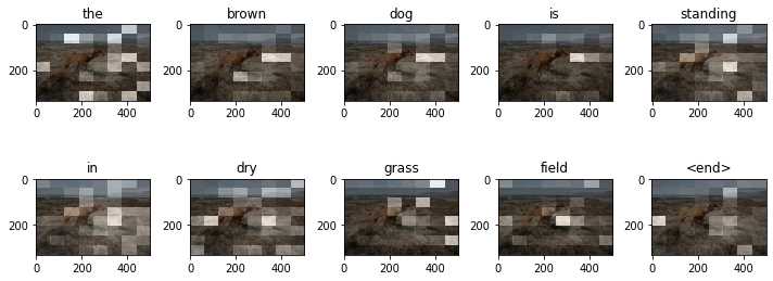
Image.open(img_name_val[r])
You can also try this code with Online Python Compiler
Real Caption: brown dog in field
Prediction Caption: the brown dog is standing in dry grass field
time took to Predict: 2 sec
FAQs
-
What are Attention Models?
Attention models, also known as attention mechanisms, are neural network input processing strategies that allow the network to focus on specific parts of a complicated input one by one until the entire dataset is categorized.
-
What are attention layers?
The attention layers are based on human concepts of attention, however, they are just a weighted mean reduction. The query, the values, and the keys are all fed into the attention layer. When the query has one key and the keys and values are the same, these inputs are frequently identical.
-
What is the self-attention model?
The self-attention mechanism, in layman's words, allows the inputs to interact with one another ("self") and determine who they should pay more attention to ("attention"). These interactions and attention scores are aggregated in the outputs.
Key Takeaways
In this article, we have discussed the following topics:
- Attention mechanism
- Working of Bahdanau attention model
- Implementation of image captioning model
Want to learn more about Machine Learning? Here is an excellent course that can guide you in learning.
Happy Coding!


 8+ registered

