Table of contents
1.
Introduction
2.
Unrolling The Recurrent Neural Network
3.
Backpropagation Through Time
3.1.
Limitations of BPTT
4.
Frequently Asked Questions
5.
Key Takeaways
Last Updated: Mar 27, 2024

Backpropagation Through Time-RNN

Author Mayank Goyal
1 upvote
Career growth poll
Do you think IIT Guwahati certified course can help you in your career?

Introduction

First, let us briefly go over Backpropagation. Backpropagation is a training algorithm that we use for training neural networks. When preparing a neural network, we are tuning the network's weights to minimize the error concerning the available actual values with the help of the Backpropagation algorithm. Backpropagation is a supervised learning algorithm as we find errors concerning already given values.

The backpropagation training algorithm aims to modify the weights of a neural network to minimize the error of the network results compared to some expected output in response to corresponding inputs.

The general algorithm of Backpropagation is as follows:

  1. We first train input data and propagate it through the network to get an output.
  2. Compare the predicted outcomes to the expected results and calculate the error.
  3. Then, we calculate the derivatives of the error concerning the network weights.
  4. We use these calculated derivatives to adjust the weights to minimize the error.
  5. Repeat the process until the error is minimized.


In simple words, Backpropagation is an algorithm where the information of cost function is passed on through the neural network in the backward direction. The Backpropagation training algorithm is ideal for training feed-forward neural networks on fixed-sized input-output pairs.

Unrolling The Recurrent Neural Network

We will briefly discuss RNN to understand how the backpropagation algorithm is applied to recurrent neural networks or RNN. Recurrent Neural Network deals with sequential data. RNN predicts outputs using not only the current inputs but also by considering those that occurred before it. In other words, the current outcome depends on the current production and a memory element (which evaluates the past inputs).

The below figure depicts the architecture of RNN :


                               img_src

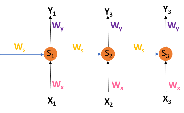
We use Backpropagation for training such networks with a slight change. We don't independently train the network at a specific time "t." We train it at a particular time "t" as well as all that has happened before time "t" like t-1, t-2, t-3.

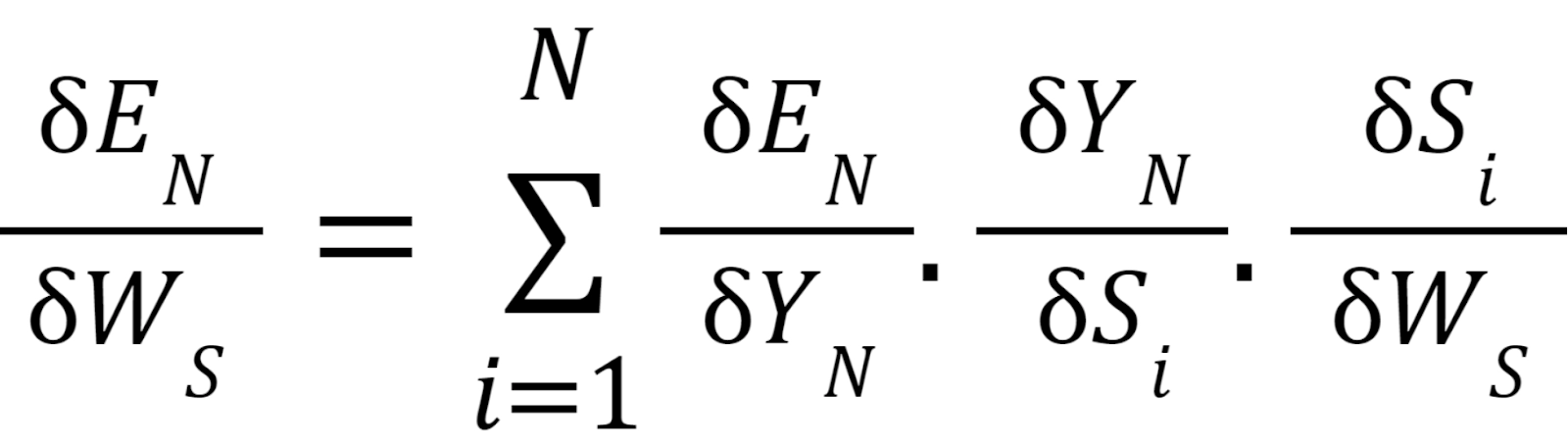
S1, S2, S3 are the hidden states at time t1, t2, t3, respectively, and Ws is the associated weight matrix.

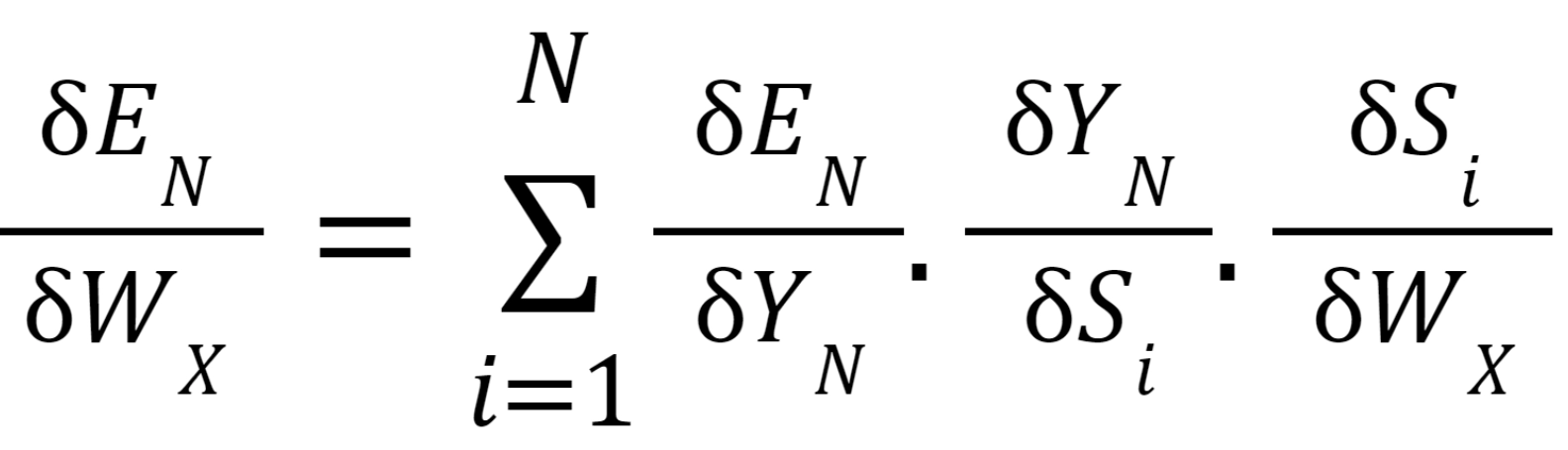
x1, x2, x3 are the inputs at time t1, t2, t3, respectively, and Wx is the associated weight matrix.

Y1, Y2, Y3 are the outcomes at time t1, t2, t3, respectively, and Wy is the associated weight matrix.

At time t0, we feed input x0 to the network and output y0. At time t1, we provide input x1 to the network and receive an output y1. From the figure, we can see that to calculate the outcome. The network uses input x and the cell state from the previous timestamp. To calculate specific Hidden state and output at each step, here is the formula:

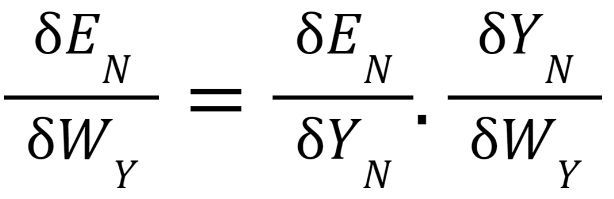
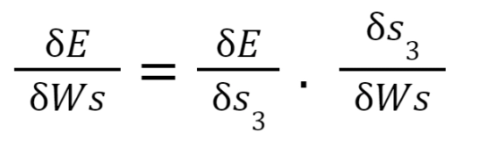
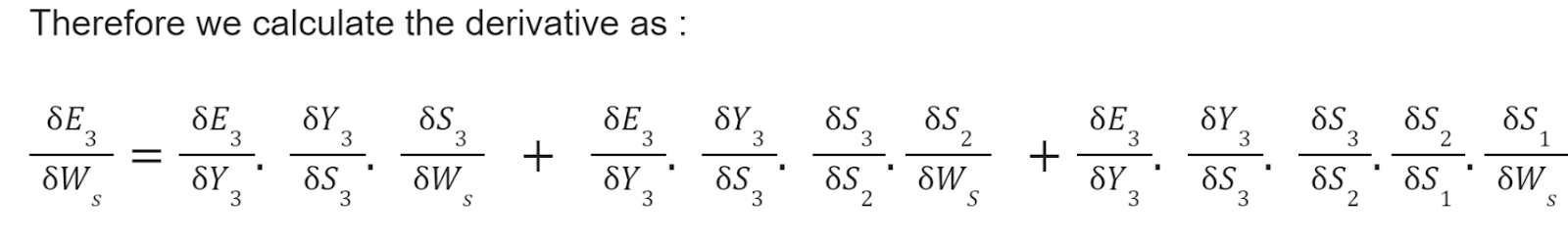
 To calculate the error, we take the output and calculate its error concerning the actual result, but we have multiple outputs at each timestamp. Thus the regular Backpropagation won't work here. Therefore we modify this algorithm and call the new algorithm as Backpropagation through time.

Backpropagation Through Time

It is important to note that Ws, Wx, and Wy do not change across the timestamps, which means that for all inputs in a sequence, the values of these weights are the same.

The error function is defined as:

Now the question arises: What is the total loss for this network? How do we update the weights  Ws, Wx, and Wy?

The total loss we have to calculate is the sum in overall timestamps,i.e., E0+E1+E2+E3+...

Now to calculate the error gradient concerning Ws, Wx, and Wy. It is relatively easy to calculate the loss derivative concerning Wy as the derivative only depends on the current timestamp values.

Formula:

But when calculating the derivative of loss concerning Ws and Wx, it becomes tricky.

Formula:

The value of s3 depends on s2, which is a function of Ws. Therefore we cannot calculate the derivative of s3, taking s2 as constant. In RNN networks, the derivative has two parts, implicit and explicit. We assume all other inputs as constant in the explicit part, whereas we sum over all the indirect paths in the implicit part.  

The general expression can be written as:

Similarly, for Wx, it can be written as:

Now that we have calculated all three derivatives, we can easily update the weights. This algorithm is known as Backpropagation through time, as we used values across all the timestamps to calculate the gradients.

The algorithm at a glance:

  • We feed a sequence of timestamps of input and output pairs to the network.
  • Then, we unroll the network then calculate and accumulate errors across each timestamp.
  • Finally, we roll up the network and update weights.
  • Repeat the process.

Limitations of BPTT

BPTT has difficulty with local optima. Local optima are a more significant issue with recurrent neural networks than feed-forward neural networks. The recurrent feedback in such networks creates chaotic responses in the error surface, which causes local optima to occur frequently and in the wrong locations on the error surface.

When using BPTT in RNN, we face problems such as exploding gradient and vanishing gradient. To avoid issues such as exploding gradient, we use a gradient clipping method to check if the gradient value is greater than the threshold or not at each timestamp. If it is, we normalize it. This helps to tackle exploding gradient.

We can use BPTT up to a limited number of steps like 8 or 10. If we backpropagate further, the gradient becomes too negligible and is a Vanishing gradient problem. To avoid the vanishing gradient problem, some of the possible solutions are:

  • Using ReLU activation function in place of tanh or sigmoid activation function.
  • Proper initializing the weight matrix can reduce the effect of vanishing gradients. For example, using an identity matrix helps us tackle this problem.
  • Using gated cells such as LSTM or GRUs.

Frequently Asked Questions

  1. Does real-time recurrent learning is faster than BPTT?
    No, BPTT tends to be significantly faster for training recurrent neural networks than general-purpose optimization techniques such as evolutionary optimization.
     
  2. What are the advantages of truncated BPTT over BPTT?
    Truncated Backpropagation Through Time (truncated BPTT) is widespread learning of recurrent computational graphs. Truncated BPTT keeps the computational benefits of Backpropagation Through Time (BPTT) while relieving the need for a complete backtrack through the whole data sequence at every step.
     
  3. What are the differences between the backpropagation algorithm and the BPTT algorithm?
    BPTT applies the Backpropagation training algorithm to an RNN applied to sequence data like a time series. An RNN is shown one input each timestep and predicts one output. Conceptually, BPTT works by unrolling all input timesteps.
     
  4. What is the BPTT algorithm?
    BPTT is the application of the Backpropagation training algorithm to recurrent neural networks applied to sequence data like a time series. 
     
  5. What are the advantages of using BPTT algorithm for training deep learning networks?
    BPTT tends to be significantly faster for training recurrent neural networks than general-purpose optimization techniques such as evolutionary optimization.

Key Takeaways

Let us brief the article.

Firstly we saw Backpropagation in a standard neural network with its algorithm, and then we discussed what's recurrent neural network is and how we update weights using Backpropagation through time. Finally, we saw some of the limitations faced by the BPTT algorithm and how do we overcome those.

That's the end of this article, where we learned how we update weights in RNN by using Backpropagation through time.

Happy Learning Ninjas!

Live masterclass