Code360 powered by Coding Ninjas X Naukri.com. Code360 powered by Coding Ninjas X Naukri.com
Table of contents
1.
Introduction  
2.
What is Recursion?
2.1.
When should we use Recursion?
2.2.
Example
2.3.
Implementation in C++
2.4.
C++
2.5.
Flowchart
2.6.
Base Case
2.7.
Time Complexity
2.8.
Space Complexity
2.9.
Advantages of Recursion
2.10.
Disadvantages of Recursion
2.11.
Applications of Recursion
3.
What is Backtracking?
3.1.
Example
3.2.
Backtracking Approach
3.3.
Algorithm
3.4.
Dry Run
3.5.
Implementation in C++
3.6.
C++
3.7.
Visualisation
3.8.
Time Complexity
3.9.
Space Complexity
3.10.
Advantages of Backtracking
3.11.
Disadvantages of Backtracking
3.12.
Applications of Backtracking
4.
What is the difference between Backtracking and Recursion?
5.
Frequently Asked Questions
5.1.
What do you understand by space complexity?
5.2.
How can we calculate the time complexity of a program?
5.3.
What is an application of recursion?
5.4.
What is one application of backtracking?
5.5.
What is the time complexity of Backtracking problems?
6.
Conclusion
Last Updated: Mar 27, 2024
Medium

Difference between Backtracking and Recursion

Introduction  

Hello ninjas. In this blog, we will discuss the concepts of backtracking and recursion and will also see the contrast between them. Recursion and backtracking are two of the most crucial algorithms and techniques for solving various problems. 
Backtracking and Recursion

Recursion can massively reduce the length and complexities of our code and is a more optimal approach against iteration. All sorts of tree and graph traversals and the famous Euclid's GCD(Greatest Common Divisor) can be efficiently done using recursion.

Backtracking is a technique which involves recursively finding solutions to a problem. It undoes the recursive changes if conditions are not met while discarding the less optimal ones to arrive at the best solution. It is a way more efficient technique than brute force. Though exponential in time complexity, backtracking is a fascinating approach that can easily solve the most complex problems of N-Queen and TSP(Travelling salesman problem).

Now, let's learn more about these techniques and conclude their differences.

What is Recursion?

Recursion is a phenomenon in computer science where a particular algorithm is repeated until it reaches its base case. In other words, when a function calls itself, it's called recursion.

It would be a lot simpler for the ones who have seen the movie Inception to understand the concept of recursion. As seen in the movie, Leonardo ambiguously has a dream. The character then has a dream inside the dream and has yet another dream, and this chain continues. 

This can be theorised by taking a function dream() and repeatedly calling itself to eternity.

void dream()
{
    cout << "Dream inside a dream" << endl;
    dream();
}


Recursion follows a similar concept of a function repeatedly calling itself until it arrives at the base case.

When should we use Recursion?

Recursion is best used when a problem can be broken down into smaller, similar subproblems. It's particularly useful when the problem can be solved by solving smaller instances of the same problem. Use recursion when the problem naturally exhibits a recursive structure, such as tree traversal, divide and conquer algorithms, or problems that involve backtracking. However, it's important to consider the potential drawbacks of recursion, such as stack overflow for deeply recursive calls, and in some cases, recursion might not be the most efficient solution compared to iterative approaches.

Example

Recursion is used in solving problems that can break into smaller sub-problems of a similar kind. Let's take a simple example to understand how recursion functions. Let us find the factorial of a number.

Implementation in C++

  • C++

C++

#include<bits/stdc++.h>
using namespace std;
int factorial(int x) {

   // Base Case
   if (x == 0)
   {
       return 1;
   }
   
   // Recursively calling the function
   return x * factorial(x - 1);
}

// Driver Code
int main() {
   int n;
   cout<<"Enter the number: ";
   cin>>n;
   cout<<"Factorial of the number= "<<factorial(n);
   return 0;
}
You can also try this code with Online C++ Compiler
Run Code


Output:

output of recursion

Flowchart

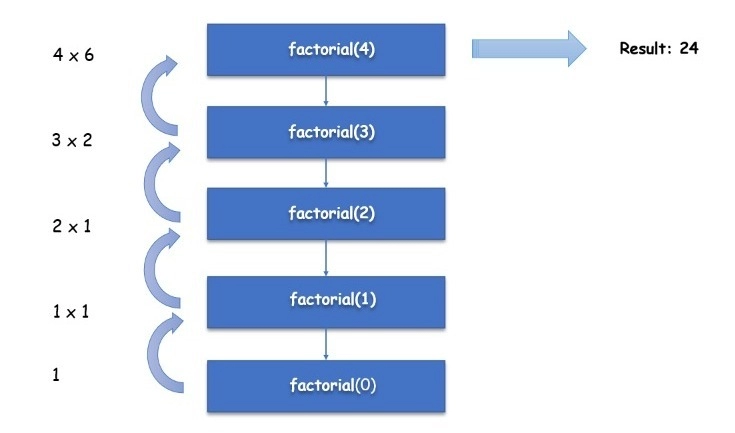
The flow chart shows how recursion works for factorial(4):
flowchart for factorial

Base Case

Every recursive function has a terminating condition called the base case. The base case condition is the one for which the answer is already known, we know the answer for that condition, and we need to return it. 

So here, in this problem, we know that factorial(0) = 1, so when x is equal to zero, we return one. 

Else we break into smaller sub-problem, i.e., factorial(x-1). 

If we don't include the base case, the function will keep calling itself and never end.

Time Complexity

For the base, the time complexity, i.e., the time complexity f(0), is 1, which can be computed in 1 unit of time because there is only one comparison. 

Still, in the general case for factorial(n), there is only one comparison and, one multiplication, one subtraction. Therefore, the time complexity can be computed in 3 units of time.

So the recurrence relation can be written as:

T(n) = 1  {where, n=0}

and          

T(n) = T(n-1) + 3

        = T(n-2) + 6

        = T(n-3) + 9

        = ….. 

       = T(n-k) + 3k

Substitution method:

If k=n, then, 

T(n) = T(0) + 3n, (as, k=n)

        = 1 + 3n

Therefore, the time complexity is O(n).

Space Complexity

For every call in the recursive function, the call is saved in the program stack till the value is computed and returned to the function.

f(5) → f(4) → f(3) → f(2) → f(1) → f(0)

f(5) → f(4) → f(3) → f(2) → f(1)

f(5) → f(4) → f(3) → f(2)

f(5) → f(4) → f(3)

f(5) → f(4)

f(5)

As you can see from the above picturisation, the f(5) will require a stack of size five to store all the calls from 5 to 1. 

Since n calls will be stored at max in the stack, the space complexity would be O(n). 

Advantages of Recursion

The advantages of Recursion are:

  • Concise code: Recursion can lead to more elegant and concise solutions, especially for problems with recursive structures.
  • Simplified logic: It often simplifies the logic of algorithms by allowing the problem to be broken down into smaller, more manageable parts.
  • Handling nested structures: Recursion is well-suited for handling nested data structures like trees and graphs.\
  • Facilitates divide and conquer: It's integral to the divide and conquer paradigm, making it useful for solving problems like sorting and searching.

Disadvantages of Recursion

The disadvantages of Recursion are:

  • Stack overflow: Deeply recursive functions can lead to stack overflow errors due to the limited size of the call stack.
  • Performance overhead: Recursion can introduce performance overhead compared to iterative solutions due to function calls and stack manipulation.
  • Debugging complexity: Recursive functions can be harder to debug and understand, especially when dealing with multiple recursive calls and base cases.
  • Memory consumption: Recursive function calls consume additional memory for maintaining the call stack, which might not be efficient for large problem instances.

Applications of Recursion

The applications of Recursion are:

  • Tree and graph traversal: Recursion is commonly used for traversing tree and graph structures, such as in depth-first search and tree traversal algorithms.
  • Dynamic programming: Many dynamic programming algorithms involve recursion to break down a problem into smaller subproblems and memoize the results.
  • Backtracking: Recursive backtracking algorithms are used to exhaustively search for solutions to combinatorial problems like the N-queens problem or Sudoku.
  • Divide and conquer: Recursion is fundamental to divide and conquer algorithms like merge sort, quicksort, and binary search, which exploit the recursive nature of the problem to efficiently solve it.

What is Backtracking?

Backtracking is a technique which involves recursively finding solutions to a problem. It undoes the recursive changes if conditions are not met while discarding the less optimal ones to arrive at the best solution. 

We break the problem down into smaller sub-problems. We check if that solution does or does not fulfill our needs, backtrack to our main problem, and check for other smaller sub-problems. We solve every problem, one piece at a time and discard the solutions that do not satisfy the problem's constraints.

Example

Let's understand backtracking with an example. 

N-Queen’s Problem: We are given a chessboard of size NxN, and we need to place N queens so that no queen attacks the other queens. Queen can attack in three directions: vertical, horizontal and diagonal.

You can check out How to Solve 8 Queens Problem Using Backtracking here.

Backtracking Approach

We will place queens in different columns one by one, starting from the leftmost column. After placing a queen in a column, we will check if any previously placed queen is clashing with this queen. 

If we find any row in the current column with no clash, we will place the queen there and mark this row and column. 

If we do not find any row in a particular column where a queen can be placed, then the solution does not exist for this chessboard of size N, and we will backtrack and return false.

Algorithm

  1. We will start with the leftmost column.
     
  2. If all queens get placed, we will return true.
     
  3. We will try all the rows in the current column one by one.
    • If the queen is safe on this row, mark this row and column in the solution, and then check if placing a queen here will lead to a solution.
       
    • If placing a queen on this cell leads to a solution, we will return true.
       
    • If placing a queen on this cell does not lead to a solution, we will unmark this cell (backtrack) and repeat the first step.
       
  4. If all rows have been checked and we didn't find any solution, we will return false to the primary function.

Dry Run

The following illustrations will help you understand the working of the algorithm in a 4×4 Chessboard.

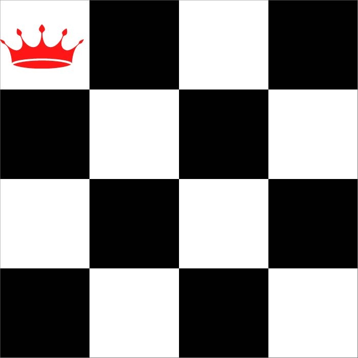
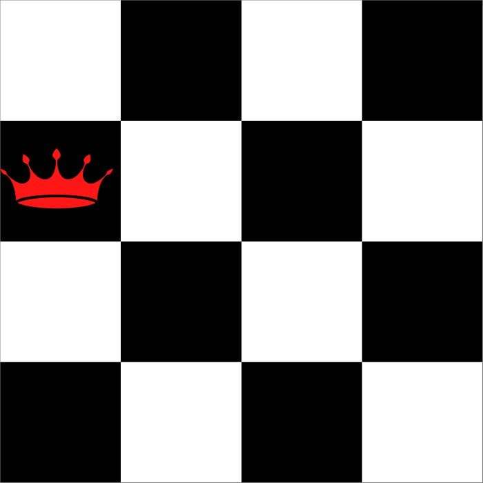
  • We place the queen in the leftmost column of our chessboard.
first queen at {1, 1}
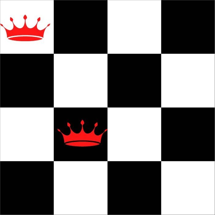
  • Now, we will place the second queen in the second column without being attacked by the previously placed queen.
second queen at {3, 2}
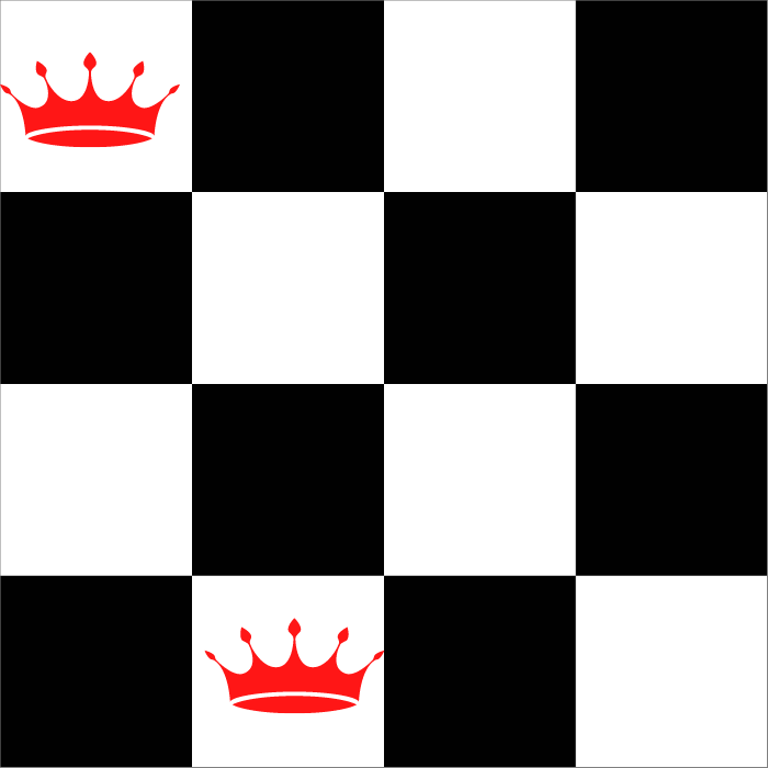
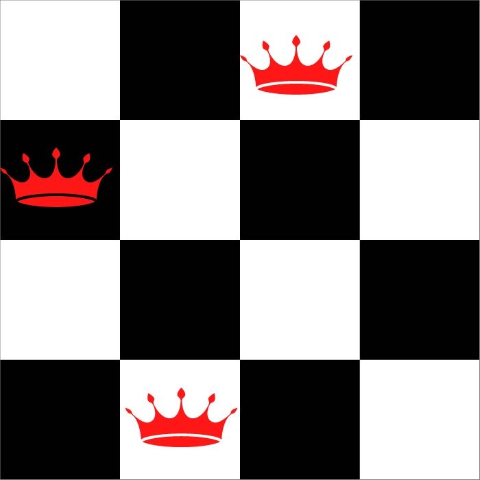
  • Now, we will place the third queen without being attacked by the previously placed queens. As one will realise, placing the third queen is impossible. Hence, we will backtrack to replace the second queen.
second queen at {4, 2}
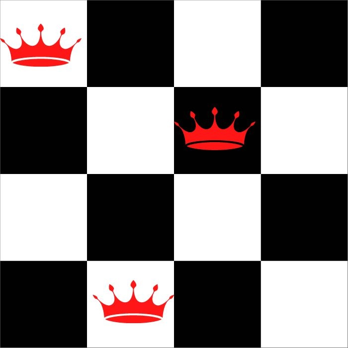
  • We will now place the third queen in the second row of the third column.
third queen at {2, 3}
  • Now, we will place the fourth queen without being attacked by the previously placed queens. Once again, it is not possible to place the queen safely. Hence, we will now backtrack to replace the first queen. We will place the first queen in the second row of the first column.
first queen at {2, 1}
  • Now, we will place the second queen in the safe row of the second column.
second queen at {4, 2]
  • Similarly, let’s place the third and fourth queens in the third and fourth columns, respectively.
third queen at {1, 3}
fourth queen at {3, 4}
  • This is our final result.

Implementation in C++

  • C++

C++

#include <bits/stdc++.h>
using namespace std;

/*
   This function will check if the queen will clash
   with any previously placed queens in any
   row or column.
*/
bool notClash(int board[][4], int row, int column)
{
   int i, j;
   /*
       To check the left column
   */
   for (i = 0; i < column; i++)
       if (board[row][i] != 0)
           return false;
   /*
       To check the upper left diagonal
   */
   i = row, j = column;
   while(i >= 0 && j >= 0){
       if (board[i][j] != 0)
           return false;
       i--;
       j--;
   }
   /*
       To check the lower diagonal of the left side
   */
   i = row, j = column;
   while(i <4 && j >= 0){
       if (board[i][j] != 0)
           return false;
       i++;
       j--;
   } 
   /*
       If the queen does not clashes with any
       previously placed queens
   */
   return true;
}

/*
   This function will solve the N-Queen Problem
*/   
bool solve(int board[][4], int column)
{
   // Base case
   if (column >= 4)
       return true;

   /*
       We will need to check every row of every column
       one at a time.
   */
   for (int i = 0; i < 4; i++)
   {
   /*
       Now, we will use notClash() function
       to check if the queen can be placed on board[i][column]
       without clashing with any other queen.
   */   
       if (notClash(board, i, column))
       {
           // Place the queen on board[i][column]
           board[i][column] = 1;

           /*
               Now we will perform recursion and call the
               function again to solve for the rest of
               the queens.
           */   
           if (solve(board, column + 1))
               return true;

           /*
               If placing a queen on this co-ordinate
               does not lead to a solution then
               remove the queen from this co-ordinate
               and backtrack to the previous column.
           */
           board[i][column] = 0;
       }
   }

   // If the queen is impossible to be placed
   return false;
}

// Driver code
int main()
{
   int board[4][4] = {{0, 0, 0, 0},
                      {0, 0, 0, 0},
                      {0, 0, 0, 0},
                      {0, 0, 0, 0}};

   /*
       If this function returns false then
       the solution does not exist.
   */
   if (solve(board, 0) == false)
   {
       cout << "Queens cannot be placed";
   }
   else
   {
       /*
           If the queen is placed on any cell
           then that cell would have a value of 1.
       */
       for (int i = 0; i < 4; i++)
       {
           for (int j = 0; j < 4; j++)
               cout << board[i][j] << " ";
           cout << endl;
       }
   }
}
You can also try this code with Online C++ Compiler
Run Code


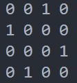
Output:

output of backtracking

Visualisation

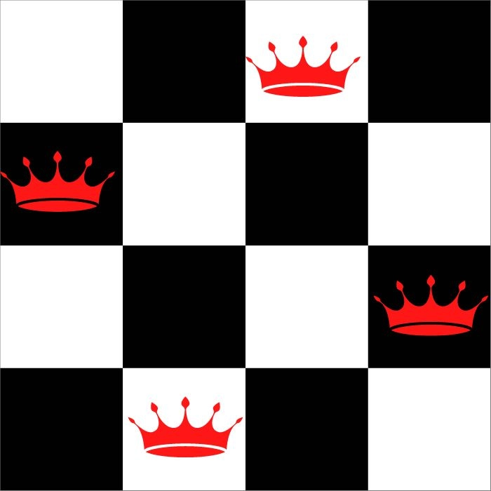
For N=4, the output can also be visualised as 

visualisation of n-queen 1

This is similar to the output received from our code, which is visualised as: 

visualisation of n-queen 2

Time Complexity

The time complexity of the N-Queen problem is ‘O(n^2)’. As we have only two choices for each queen, i.e., we can either place or not place it at a certain position.

Space Complexity

The space complexity of the N-Queen problem is ‘O(n^2)’, where ‘n’ denotes the number of queens. This is due to the usage of a 2-D array which will have a linear space due to the recursion.

Advantages of Backtracking

The advantages of Backtracking are:

  • Versatile approach: Backtracking is a flexible technique applicable to a wide range of problems, including constraint satisfaction, combinatorial optimization, and decision-making.
  • Memory efficiency: It typically requires less memory compared to other exhaustive search techniques because it explores solutions incrementally and discards unsuccessful paths.
  • Solution space pruning: Backtracking intelligently prunes the search space by abandoning partial solutions that cannot lead to a valid solution, thereby improving efficiency.
  • Elegant solution representation: It allows for elegant and concise representations of problems, especially those involving constraints and decisions, making the code easier to understand and maintain.

Disadvantages of Backtracking

The disadvantages of Backtracking:

  • Exponential time complexity: In worst-case scenarios, backtracking algorithms can have exponential time complexity, especially for problems with large search spaces or weak constraints.
  • Difficulty in optimization: It can be challenging to optimize backtracking algorithms, particularly when dealing with complex decision spaces or heuristic-based pruning strategies.
  • Potential inefficiency: In some cases, backtracking may explore a significant portion of the search space before finding a solution, leading to inefficiencies, especially for problems with sparse solutions.
  • Implementation complexity: Implementing backtracking algorithms correctly requires careful handling of state transitions, termination conditions, and solution space exploration, which can lead to complex code.

Applications of Backtracking

The applications of Backtracking are:

  • N-queens problem: Backtracking is commonly used to find all possible arrangements of queens on an N×N chessboard such that no two queens threaten each other.
  • Sudoku solving: Backtracking algorithms efficiently explore possible solutions for completing partially filled Sudoku grids while adhering to the rules of the game.
  • Constraint satisfaction problems: Backtracking is widely employed in constraint satisfaction problems like the map coloring problem, job scheduling, and resource allocation.
  • Cryptarithmetic puzzles: Backtracking techniques are used to solve cryptarithmetic puzzles, where letters represent digits and arithmetic operations need to be satisfied to form a valid equation.

What is the difference between Backtracking and Recursion?

Sl. No. Recursion Backtracking
1. Backtracking is only sometimes required to do recursion.  Recursion is always necessary to do backtracking.
2. It is comparatively more straightforward. It is comparatively more complex.
3. Recursion involves a function repeatedly calling itself until it arrives at the base solution. Backtracking involves finding solutions one at a time and discarding the less optimal ones at every step.
4. Applications include, Graph and tree traversals like DFS, Postorder, preorder and merge sort, quick sort etc. Applications include complex problems like N-Queen, Rat-in-a-maze, Travelling Salesman and graph colouring.

Check this out, Yarn vs NPM

Frequently Asked Questions

What do you understand by space complexity?

The space complexity of a program can be defined as the total space taken in the memory by the algorithm with respect to its input.

How can we calculate the time complexity of a program?

An algorithm's time complexity can be computed using substitution or recursive tree methods.

What is an application of recursion?

Many well-known sorting algorithms (Quick sort, Merge sort, etc.) use recursion.

What is one application of backtracking?

The travelling salesman problem is a salesman wants to travel all the cities on a map only once. He must find the optimal path to reach every town before crossing a city twice.

What is the time complexity of Backtracking problems?

The backtracking problems generally have an exponential time complexity of ‘O(k^n)’, where ‘k’ is the number of times the function calls itself and n is the time spent doing the work on each function.

Conclusion

In this article, we discussed the difference between Backtracking and Recursion. While backtracking and recursion share similarities, they serve distinct purposes in algorithmic problem-solving. Recursion is a general programming concept that involves a function calling itself to solve smaller instances of a problem, often leading to elegant and concise solutions. On the other hand, backtracking is a specific algorithmic technique used to systematically explore potential solutions, especially in constraint satisfaction and combinatorial optimization problems.

You can refer to this to learn more about backtracking and recursion.

  1. Backtracking
  2. Recursion
     

Never stop learning. Explore more here.

For placement preparations, you must look at the problemsinterview experiences, and interview bundles. Enrol in our courses and refer to the mock tests and problems available; look at the Problem Sheetsinterview experiences, and interview bundle for placement preparations. You can also book an interview session with us.  

Recommended Problems:

Consider our paid courses, to give your career a competitive advantage! Until then, keep learning and keep practicing on Code studio.

Happy Coding!

Live masterclass