Basic Execution Time Model

Introduction

There are multiple types of software available with the same functions, yet some of them work well and are capable of retaining their users, and some of them lose their users over time. So why is there a difference? 

One of the reasons is continuously working on the failures and errors, and the other is not doing so. So how is some software being tested?

To solve the above problem, there are many methods available, and the basic execution time model is one of them. We will discuss it while moving further in the blog, so let's get on with our topic without wasting any time.

Basic Execution Time Model Explanation and Equations

This is also known as the Musa model, as in 1979, J.D. Musa proposed it.

The basic execution model is generally, and the most popular used reliability growth model is usually used.

Features

There are many features of the basic execution time model which make it perfect for use. We will discuss some of them here.

• It is simple, practical, and easy to understand.
• Its parameters are easy to understand as they directly relate to the physical world.
• We can use it for accurate reliability prediction.

As the name suggests, it determines the failure by using the execution time. We can convert execution time into calendar time according to requirements.

The failure is a nonhomogeneous Poisson process. We understand from the previous statement that associated probability distribution is a Poisson process, and its characteristics vary in time.

We can conclude from the above statement that the mean value function will be exponential distribution.

Equations

Failure intensity(λ): The number of failures per unit time is measured.

Mean failure experienced(μ): It is a mean failure experienced in a unit time interval.

Execution Time(τ): The time since the program is running.

Where 

-λ₀: At the start of execution, it stands for initial failure intensity.

υ_0: It determines the total number of failures occurring in an infinite period. It can be said that the total number of failures is to be considered.

We can express failure intensity as a function of execution time as follows:

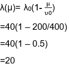
Expressing failure intensity in terms of μ below:

Where

λ₀: initial

υ_0: Number of failures in infinite time. 

μ: Expected or the average number of failures in a given time interval.

τ: Execution Time.

Source

                                          Source

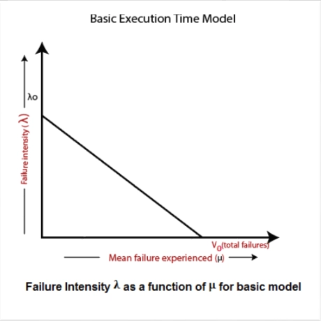
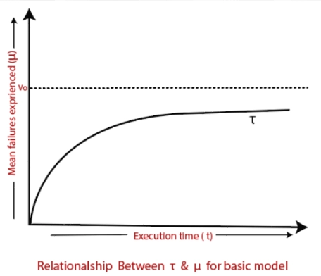
In the derivative form, we can write equation one as:

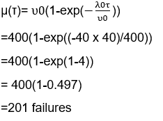
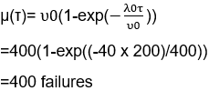
By solving the above equation, we get the following result:

The failure intensity as a function of execution time is shown below:

                                            Source

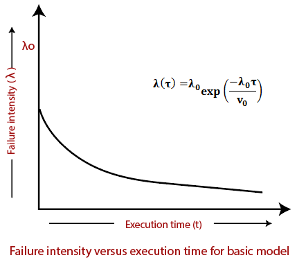
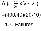
Computing the number of failures with given failure intensity will be shown as below:

                                         Source

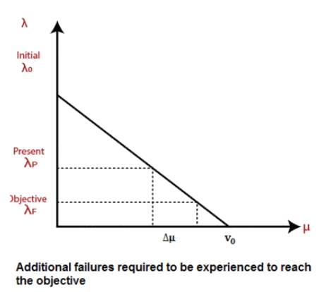
Where

λ₀: Initial failure intensity.

λ_P: Present failure intensity

λ_F: Failure of intensity objective.

Δ μ: Expected number of failures to be experienced while working.

                                         Source

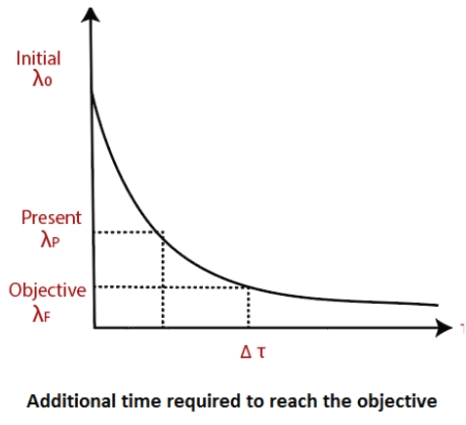
Writing the above graph in the mathematical form will look like this:

Also see,  V Model in Software Engineering