Baum Welch Algorithm - HMM

Introduction

Hidden Markov Model is a concept in Machine Learning which uses the concept of Cumulative Reward, which follows a sequence of observations to train by itself and come to a decision or conclusion. We can also define this as a statistical approach used to describe the evolution of observations that depends on internal factors or internal decisions.

You can introduce yourself to the concept of HMM and use-case of it by going through Introduction to HMM.

We have Viterbi Algorithm, a dynamic programming approach to optimize an HMM model's paths in its preparation. Similarly, another technique used to optimize the parameters needed to be taken by an HMM model is called Baum Welch Algorithm.

Baum Welch Algorithm

Baum Welch Algorithm, an optimization approach, uses both dynamic programming approach and the concept of Expectation-Maximisation (EM) algorithm.
The Baum Welch Algorithm is also called as "Forward-Backward Algorithm. As we already know that an HMM matrix will include the terms the Transition matrix and the Emission Matrix. The Estimation Step in this algorithm will estimate these two matrices and maximize the final likelihood result. Baum Welch Algorithm is essentially used to optimize or tune the HMM model parameters. This can be done by a special use-case of the Expectation-Maximisation technique.
In the view of Expectation-Maximisation, The algorithm will look like this,

Step1: Will Begin with some model μ,  μ = (T, E)
where T = Transition Probability Matrix, and E = Emission Probability Matrix.
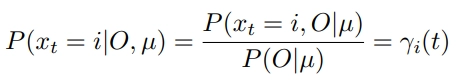
Here we need to find P(x_t  = i, O|μ )

Step2: Run the Observation O through the developed or current model to estimate the expectations of each parameter of the HMM model. This will be considered as E-step.

Step3: Update the model to maximize the parameters of the paths used a lot by keeping an eye on the stochastic constraints. This will be considered as our M-step.

Step4: Repeat until we reach the optimal values for the model parameters, μ.
In the view of the Forward-Backward Algorithm concept, 
To understand this algorithmic view, first, we will take an eye on the optimized or output parameters of the HMM model using this Baum Welch Algorithm.

Here a* and b* are the optimized transition and emission probability matrices(parameters of the HMM model.
Now we can easily understand the steps in this algorithm,

Step1: This is an initial step, where we will initialize the parameters a, b as the transition and emission probability matrices.

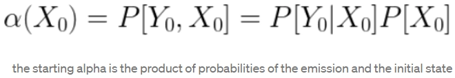
Step2: This will be our forward phase where we will concentrate on developing an alpha function recursively; this alpha function will look as shown below:
The initial alpha function will look as 

Then this alpha will develop recursively as,

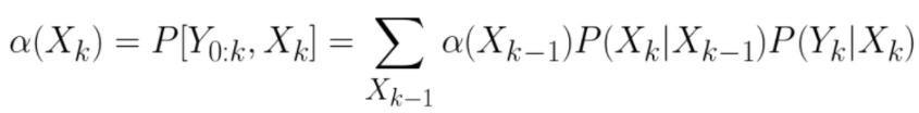
Where the value k refers to the unit of the current time, this alpha function will be defined as the joint probability function of the observed events up to time k(Y) and the state at time k(X).
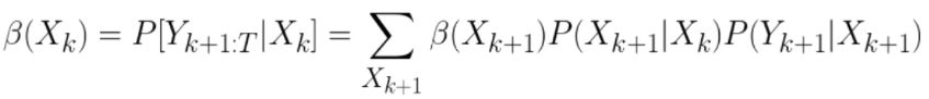
Step3: This step will be considered as the Backward phase. Where we will try to develop the Beta function where these developed alpha and beta functions are used to build the update phase, we develop the Xi, and the Eta function is used to construct the optimized parameters of the HMM model.
The initial Beta function will look as β(X_T) = 1.
Then the Beta function will develop recursively as follows,

Step4: In this step, we try to develop the Eta and Xi functions to update the parameters.
This phase can be done by using,

And then, using these developed η, ξ functions, we can develop the optimized a,b parameters for our HMM model.