Bayesian Estimation
Source - link
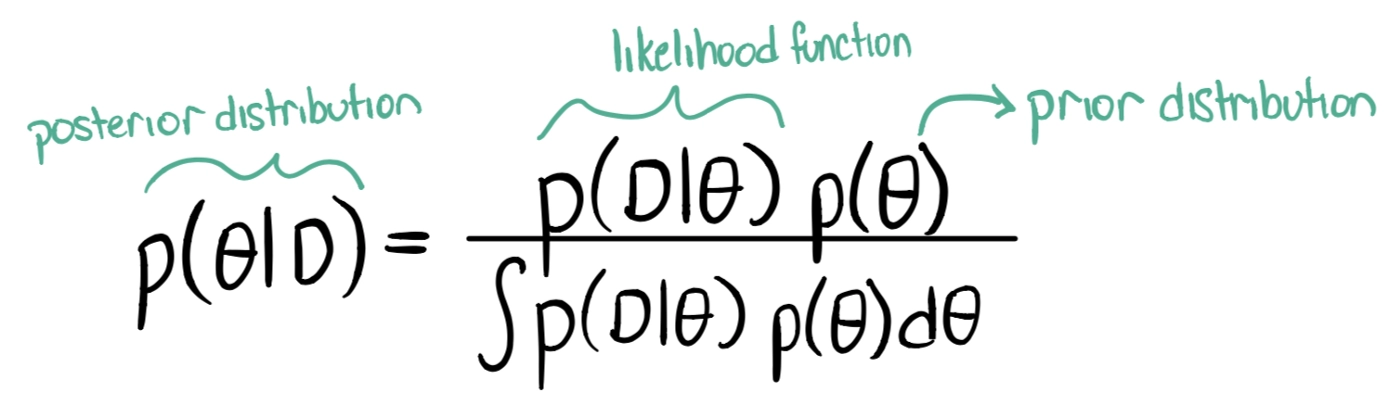
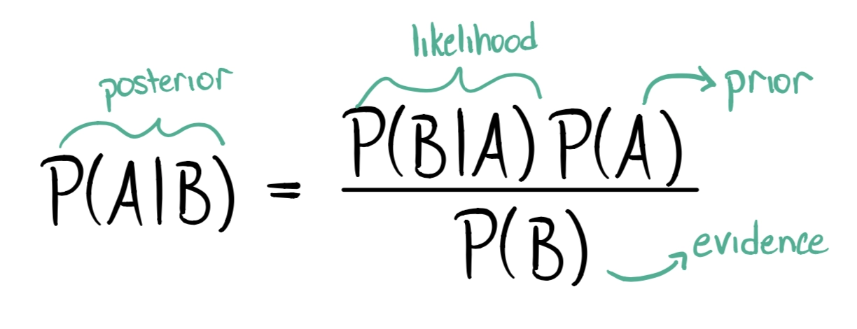
In Bayesian Estimation, the equation just takes probability distributions instead of numeric values unlike what we learned in Bayesian Decision Theory.
Notice we replaced evidence with the integral of the numerator. This is because P(D) is tough to calculate and it doesn’t depend on P(θ). It also ensures the integral of the posterior distribution to be 1.
Here ∫P(D|θ)P(θ)dθ is known as evidence.
In Bayesian Estimation, we compute a distribution over a parameter space known as posterior pdf( P(θ|D) ).
Source - link
We see that Bayesian estimation tries to encompass both, the prior probability and the likelihood function to give out the result of the posterior distribution.
Applications
- Bayesian Estimation is used to monitor cracks in gas piping systems that pose serious hazards if not handled with utmost care. The most probable parameters are estimated corresponding to cracks using prior knowledge of standard leaks.
- Bayesian estimation is used in daily clinical practice to estimate the real-time condition of a patient using prior knowledge to give the most suitable treatment.
Implementation
%matplotlib inline
import numpy as np
import pandas as pd
import statsmodels.api as sm
import sympy as sp
import pymc
import matplotlib.pyplot as plt
import matplotlib.gridspec as gridspec
from mpl_toolkits.mplot3d import Axes3D
from scipy import stats
from scipy.special import gamma

from sympy.interactive import printing
printing.init_printing()

You can also try this code with Online Python Compiler
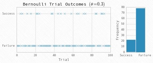
# Simulate data
np.random.seed(123)

nobs = 100
theta = 0.3
Y = np.random.binomial(1, theta, nobs)
You can also try this code with Online Python Compiler
# Plot the data
fig = plt.figure(figsize=(7,3))
gs = gridspec.GridSpec(1, 2, width_ratios=[5, 1])
ax1 = fig.add_subplot(gs[0])
ax2 = fig.add_subplot(gs[1])

ax1.plot(range(nobs), Y, 'x')
ax2.hist(-Y, bins=2)

ax1.yaxis.set(ticks=(0,1), ticklabels=('Failure', 'Success'))
ax2.xaxis.set(ticks=(-1,0), ticklabels=('Success', 'Failure'))

ax1.set(title=r'Bernoulli Trial Outcomes $(\theta=0.3)$', xlabel='Trial', ylim=(-0.2, 1.2))
ax2.set(ylabel='Frequency')

fig.tight_layout()
You can also try this code with Online Python Compiler
The likelihood function
t, T, s = sp.symbols('theta, T, s')

# Create the function symbolically
likelihood = (t**s)*(1-t)**(T-s)

# Convert it to a Numpy-callable function
_likelihood = sp.lambdify((t,T,s), likelihood, modules='numpy')
You can also try this code with Online Python Compiler
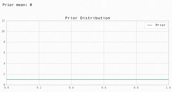
Prior
# For alpha_1 = alpha_2 = 1, the Beta distribution
# degenerates to a uniform distribution
a1 = 1
a2 = 1

# Prior Mean
prior_mean = a1 / (a1 + a2)
print('Prior mean:', prior_mean)

# Plot the prior
fig = plt.figure(figsize=(10,4))
ax = fig.add_subplot(111)
X = np.linspace(0,1, 1000)
ax.plot(X, stats.beta(a1, a2).pdf(X), 'g')

# Cleanup
ax.set(title='Prior Distribution', ylim=(0,12))
ax.legend(['Prior'])
You can also try this code with Online Python Compiler
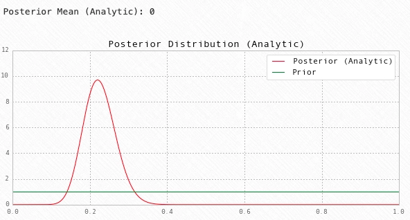
Posterior
# Find the hyperparameters of the posterior
a1_hat = a1 + Y.sum()
a2_hat = a2 + nobs - Y.sum()

# Posterior Mean
post_mean = a1_hat / (a1_hat + a2_hat)
print('Posterior Mean (Analytic):', post_mean)

# Plot the analytic posterior
fig = plt.figure(figsize=(10,4))
ax = fig.add_subplot(111)
X = np.linspace(0,1, 1000)
ax.plot(X, stats.beta(a1_hat, a2_hat).pdf(X), 'r')

# Plot the prior
ax.plot(X, stats.beta(a1, a2).pdf(X), 'g')

# Cleanup
ax.set(title='Posterior Distribution (Analytic)', ylim=(0,12))
ax.legend(['Posterior (Analytic)', 'Prior'])
You can also try this code with Online Python Compiler
FAQs
-
When do we prefer using bayesian estimation over MLE?
Computing Bayesian Estimation is a little more complex than MLE as it requires knowledge of prior, likelihood function, and evidence.
-
What are the advantages of Bayesian Estimation?
Bayesian Estimation is suited for huge data. And the variance is almost negligible.
-
What are the disadvantages of Bayesian Estimation?
Bayesian Estimation requires knowledge of a lot of other factors like prior, likelihood, and evidence. A good estimation is achieved only when we have an accurate knowledge of all the factors involved, which can be tough to gather.
Key Takeaways
Bayesian Estimation is another popular parameter estimation technique besides maximum likelihood estimation. This blog gives a beginner’s insight into the technique while contrasting it with Maximum likelihood Estimation at some points. It’s recommended for readers to go through the blog atleast a few couple times to get a better understanding of the little details that you might miss out on initially. You may check out our industry-oriented machine learning courses curated by industry experts.


 9+ registered

