Do you think IIT Guwahati certified course can help you in your career?
Introduction
Those who have come across reinforcement learning(RL) are well aware that the Bellman Equation is an unavoidable part of RL whose application can be found throughout RL in one form or the other. The Bellman equation helps generate more calculated and better-bearing results by combining different RL functions.
Before we dive deep into the Bellman equation, let’s learn some basics for understanding its application in a better way.
Understanding The Essential Keywords
1. Agent(A): The term agent is referred to the entity that performs the actions in a given environment.
2. Environment(): The environment can be defined as a situation under observation in which our agent is working.
3. State(S): The state can be defined as the result after at the end of every action taken before the reward.
4. Reward(R): A reward is feedback gained after the end of the complete cycle of the agent.
5. Policy(π): The policy represented by π is used to define the motive behind the action taken by the agent in the cycle. Mathematically policy can be stated as the set of actions in a given state, giving the probability of the following action the agent will choose.
What is Markov’s Decision Process (MDP)?
As the name suggests, Markov’s decision process can be defined as the property of cumulative actions that lie in accordance with the Markov property which states that the decision taken in the given environment is the result of a positive signal generated by the system. Markov's Decision process in RL is used for decision-making with respect to long-term rewards in the current state.
In the above image, as we can see, there are a few alphabets assigned to the processes. Let’s define and understand them.
S: It is the set of all possible states in a process.
A: It is the set of all possible actions the agent can take.
R: It is the set of all possible rewards the agent can acquire at the end of a cycle
Rt+1: It is the reward obtained at a given time t.
St+1: Is the state obtained at a given time t.
Let’s understand how this works altogether.
Our decision-maker or the agent takes action in the current state, looking at the situation that moves our environment to a different state, generating rewards as the outcome. Finite MDP following Markov’s property works only in the current state and takes decisions based on the current scenario and does not depend on past actions or rewards. The agent works in the present state, working in an optimized manner for future rewards.
Two more additions to Markov's process named as the reward function R and the discount factor γ are the following additions to our equation of the MDP.
The reward function signifies the total number of rewards attained at the end of the cycle, and Gamma shows the discount rate where 0<γ≤1.
Gama is used to make the future less uncertain; thus, the gamma is used to limit the contribution of the future rewards in our cycle.
The Markov reward process(MRP) in terms of RL evaluates the most optimized pathway to travel through the basis of maximum rewards attained. The formulae we use for the reward are shown below.
As we can see in the image above, each path or state that the agent takes has either positive or negative rewards based on what the agent does after waking up. The same is used to calculate the reward of the whole cycle, and the most optimized path is computed using the above-stated MDP formulae.
In reinforcement learning, we use value functions along with MDP to categorize the best action that one agent should perform in a given environment to attain maximum reward. Let's have a look at how these value functions look and later in this article we would be studying in depth about them.
Now that we are aware of what state-value function and action-value function look like and how they help the agent predict and find the most optimized beneficial move that the agent can make to attain better reward, let's learn in depth about them.
State-Value Function
State-Value function talks about the function of the state that deals with the long-term value of the state i.e., it helps predict the long-term reward from the current that would be obtained from the whole cycle by the agent. Let’s understand this with the help of a formula.
Where Vπ (s) represents the value function under a state
Eπ represents the expected state-value in the given time t.
In the case of the state value function, the function Vπ (s) defines how suitable the state is to be for the agent at the given time t with current state s following the policy π.
Action-Value Function
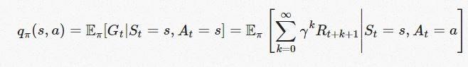
The action-value function returns the value of the action taken in the current state that follows the policy π. It signifies how beneficial it would be for the agent to take the probable action in the current state, which gives the most beneficial return and better rewards.
Where qπ (s, a) represents the action and the state
Eπ represents the stochasticity in the environment
The formulae are used to calculate the probable reward that the agent will get on taking action in the state that helps us determine the quality of the action.
Optimal Policy
The optimal policy talks about the maximum number of rewards that the agent can secure by taking the right actions in the current state. Algorithms in RL focuses on implementing optimal policy to the environments that follow it.
The goal of the optimal policy is to calculate the policy that would generate the most optimal rewards compared to other probable, possible policies.
What is Bellman Equation?
The Bellman equation helps provide a standard representation of all the value functions mentioned above and helps them break the problem into two simpler parts that are: immediate reward and the discounted future values corresponding to the action taken by the agent in the current state.
Below you will see the Bellman equation with all the constraints defined.
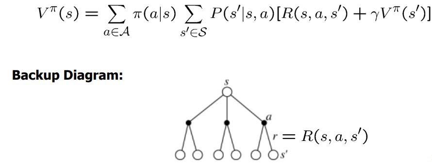
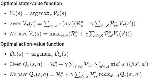
Bellman Equation For State-Value Function
Since we have already defined the state-value function before and are well aware of its functioning now, let’s understand how it works with the bellman equation.
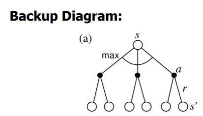
In the case of the state-value function, the bellman equation helps choose the most optimized state that followed the policy in the given environment recursively. Let’s understand it with the given formulae and backup diagram.
Here in the formulae, we can see that the Bellman equation breaks the state into two parts: the P(s`|s, a) the expected reward of the taken state and the successor with the discount rate.
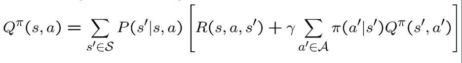
Bellman Equation For Action-Value Function
Similar to the working of the state-value function, the Bellman equation for the action-value function helps us calculate the state-action air, i.e., the state the agent is currently in, along with the expected action the agent would take in the environment.
In the formulae given below, since we are calculating both action and state pair, we take the sum of both, i.e., Q(s, a) that follows the policy π.
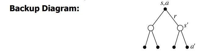
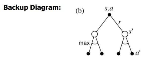
The Backup diagrams help explain the working of the active-value function for the bellman equations.
The role of the bellman optimality equation is to find the most optimal policy that the agent can follow to get the best cumulative reward when the cycle ends. Since we have already seen the state-value and active-value function in the above state, let’s move on to the optimal equation looking at the same.
This equation can be solved without the use of MDP simply by applying Bellman Equation, but usually, this doesn’t happen in our day-to-day stated problems as the value of R(s, a) and Pass` is not known.
The backup diagrams below provide us with a graphical representation of the future states and actions that our agent can achieve at the end of our cycle.
Note: The diagram on the left is for the active-value function, and that on the right is for the state-value function.
The Bellman optimality equation states, conceptually, that the reward of any state within an optimal policy has to be the return the agent receives whenever it executes the optimal policy's best action.
Optimal Policy Function
Value Functions
The policy is updated by the policy iteration algorithm. Instead of iterating over the value function. Nonetheless, in each cycle, both algorithms update the policy and state value function implicitly.
At each step, Value Iteration only performs a single iteration of policy assessment. The estimated state value is then calculated using the maximum action value for every state.
The policy iteration function has two steps in each iteration. The policy is evaluated in one phase, and improved in the other. By obtaining a maximum over the utility function for all potential actions.
The optimal policy can be determined once these state values have converged to the optimal state values. In practice, this outperforms Policy Iteration and finds the ideal state value function in a fraction of the time.
1. Shortest Path Problems: The Bellman equation is widely used in solving shortest path problems in graph theory. It allows us to find the shortest path from a starting node to all other nodes in a weighted graph. The equation iteratively updates the shortest distance to each node based on the distances of its neighboring nodes. This application is crucial in navigation systems, network routing protocols, and transportation optimization.
2. Resource Allocation: The Bellman equation finds applications in resource allocation problems, where the objective is to optimally allocate limited resources to maximize a certain outcome or minimize costs. It helps in determining the optimal allocation strategy by considering the current state and future consequences of each decision. Resource allocation problems arise in various domains, such as finance, manufacturing, and telecommunications.
3. Inventory Management: In inventory management, the Bellman equation is used to optimize inventory levels and minimize costs. It helps in determining the optimal ordering quantities and timing of orders based on factors such as demand, holding costs, and ordering costs. By applying the Bellman equation, businesses can develop efficient inventory control policies that minimize overall costs while ensuring adequate stock levels.
4. Reinforcement Learning: The Bellman equation plays a central role in reinforcement learning, a subfield of machine learning. In reinforcement learning, an agent learns to make optimal decisions by interacting with an environment and receiving rewards or penalties. The Bellman equation is used to estimate the value of each state or state-action pair, which represents the expected cumulative reward from that state onwards. It forms the foundation of various reinforcement learning algorithms, such as Q-learning and SARSA.
5. Dynamic Pricing: The Bellman equation is applied in dynamic pricing strategies, where prices are adjusted in real-time based on demand, supply, and other market conditions. It helps in determining the optimal pricing policy that maximizes revenue or profit over a given time horizon. Dynamic pricing is commonly used in industries such as airline ticket pricing, hotel room pricing, and ride-sharing services.
6. Portfolio Optimization: In finance, the Bellman equation is utilized for portfolio optimization problems. It helps in determining the optimal allocation of assets in a portfolio to maximize expected returns while considering risk constraints. The equation takes into account the current state of the portfolio, the expected returns and risks of different assets, and the investor's risk tolerance. By solving the Bellman equation, investors can make informed decisions about asset allocation and portfolio rebalancing.
7. Robotics and Control: The Bellman equation is applied in robotics and control systems to optimize the behavior of autonomous agents. It helps in determining the optimal control actions that minimize a cost function or maximize a reward function over time. The equation considers the current state of the system, the available actions, and the expected future states and rewards. This application is crucial in developing intelligent control strategies for robots, drones, and other autonomous systems.
Frequently Asked Questions
What are the real-world examples of the application of the Bellman equation?
The best examples can be seen in the finance sector, where the machine makes calculative steps to maximize the total rewards gained in a cycle. In human cognitive behavior also we can see a similar pattern where ideally humans work towards achieving the suitable reward.
Why is discount used so extensively in the MDP and Bellman Equation?
The simple answer is to have finite mathematical solutions MDP for the given cycle in an environment, reducing the uncertainty of the future.
What is the solution to the Bellman equation?
The solution to the Bellman equation involves finding a value function that satisfies the recursive relationship among states in dynamic programming, typically solved using methods like value iteration or policy iteration.
Is Bellman equation linear?
The Bellman equation is generally nonlinear due to the inclusion of maximization or minimization operators within its formulation, which are intrinsic to optimization problems in dynamic programming.
Conclusion
In this article, we have briefly discussed the mathematical application of the Bellman Equation in reinforcement learning. Bellman equation helps generate better long-term rewards in a given environment by assisting the agent in making the right move in the current state to gain better rewards in the future state.
We have also covered Markov’s Decision Process and various forms of the Bellman equation in active-value function, state value function, and the optimization policy individually and in terms of Bellman Equation in Reinforcement Learning. Learn more about reinforcement learning follow our blogs to have a better understanding of the subject.


 8+ registered

