


Introduction
To understand Bernoulli Naive Bayes algorithm, it is essential to understand Naive Bayes.
Naive Bayes is a supervised machine learning algorithm to predict the probability of different classes based on numerous attributes. It indicates the likelihood of occurrence of an event. Naive Bayes is also known as conditional probability.
Naive Bayes is based on the Bayes Theorem.
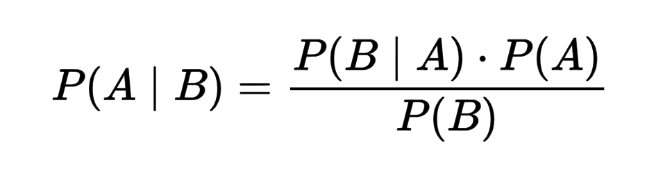
where:-
A: event 1
B: event 2
P(A|B): Probability of A being true given B is true - posterior probability
P(B|A): Probability of B being true given A is true - the likelihood
P(A): Probability of A being true - prior
P(B): Probability of B being true - marginalization
However, in the case of the Naive Bayes classifier, we are concerned only with the maximum posterior probability, so we ignore the denominator, i.e., the marginal probability. Argmax does not depend on the normalization term.
The Naive Bayes classifier is based on two essential assumptions:-
(i) Conditional Independence - All features are independent of each other. This implies that one feature does not affect the performance of the other. This is the sole reason behind the ‘Naive’ in ‘Naive Bayes.’
(ii) Feature Importance - All features are equally important. It is essential to know all the features to make good predictions and get the most accurate results.
Naive Bayes is classified into three main types: Multinomial Naive Bayes, Bernoulli Naive Bayes, and Gaussian Bayes.
We will be talking about Bernoulli Naive Bayes in this blog.
Before going ahead, let us have a look at the Bernoulli Distribution:-
Let there be a random variable 'X' and let the probability of success be denoted by 'p' and the likelihood of failure be represented by 'q.'
Success: p
Failure: q
q = 1 - (probability of Sucesss)
q = 1 - p
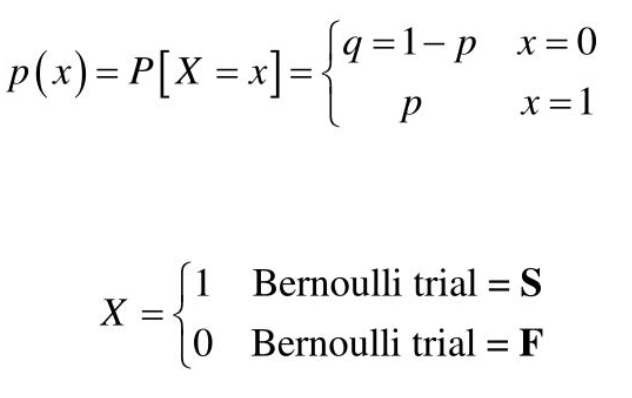
As we notice above, x can take only two values (binary values), i.e., 0 or 1.
Bernoulli Naive Bayes is a part of the Naive Bayes family. It is based on the Bernoulli Distribution and accepts only binary values, i.e., 0 or 1. If the features of the dataset are binary, then we can assume that Bernoulli Naive Bayes is the algorithm to be used.
Example:
(i) Bernoulli Naive Bayes classifier can be used to detect whether a person has a disease or not based on the data given. This would be a binary classification problem so that Bernoulli Naive Bayes would work well in this case.
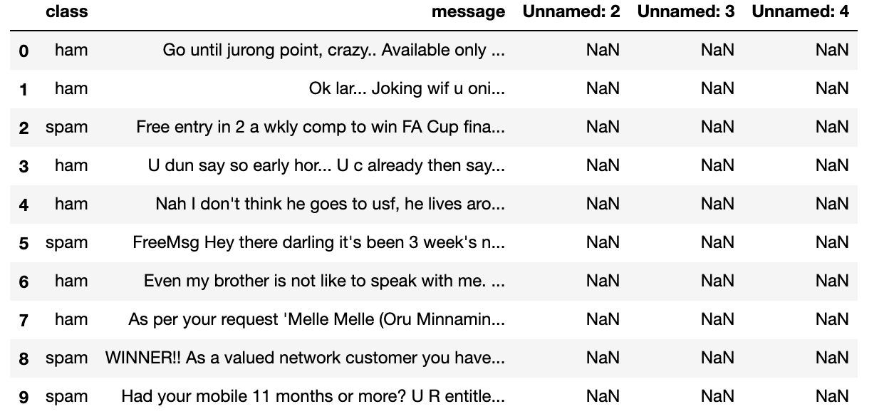
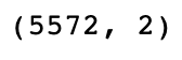
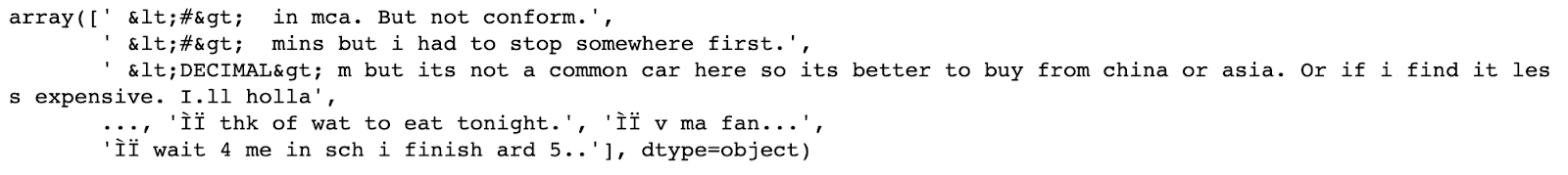
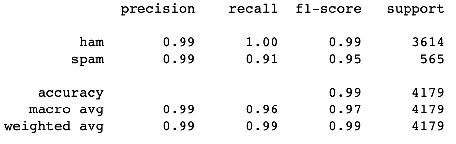
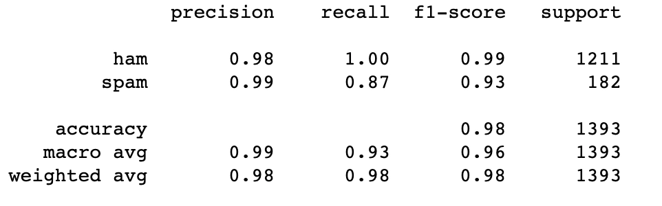
(ii) Bernoulli Naive Bayes classifier can also be used in text classification to determine whether an SMS is ‘spam’ or ‘not spam.’
Mathematics Behind
Let us consider the example below to understand Bernoulli Naive Bayes:-
| Adult | Gender | Fever | Disease |
| Yes | Female | No | False |
| Yes | Female | Yes | True |
| No | Male | Yes | False |
| No | Male | No | True |
| Yes | Male | Yes | True |
In the above dataset, we are trying to predict whether a person has a disease or not based on their age, gender, and fever. Here, ‘Disease’ is the target, and the rest are the features.
All values are binary.
We wish to classify an instance ‘X’ where Adult=’Yes’, Gender= ‘Male’, and Fever=’Yes’.
Firstly, we calculate the class probability, probability of disease or not.
P(Disease = True) = ⅗
P(Disease = False) = ⅖
Secondly, we calculate the individual probabilities for each feature.
P(Adult= Yes | Disease = True) = ⅔
P(Gender= Male | Disease = True) = ⅔
P(Fever= Yes | Disease = True) = ⅔
P(Adult= Yes | Disease = False) = ½
P(Gender= Male | Disease = False) = ½
P(Fever = Yes | Disease = False) = ½
Now, we need to find out two probabilities:-
(i) P(Disease= True | X) = (P(X | Disease= True) * P(Disease=True))/ P(X)
(ii) P( Disease = False | X) = (P(X | Disease = False) * P(Disease= False) )/P(X)
P(Disease = True | X) = (( ⅔ *⅔ * ⅔ ) * (⅗))/P(X) = (8/27 * ⅗) / P(X) = 0.17/P(X)
P(Disease = False | X) = [(½ * ½ * ½ ) * (⅖)] / P(X) = [⅛ * ⅖] / P(X) = 0.05/ P(X)
Now, we calculate estimator probability:-
P(X) = P(Adult= Yes) * P(Gender = Male ) * P(Fever = Yes)
= ⅗ * ⅗ * ⅗ = 27/125 = 0.21
So we get finally:-
P(Disease = True | X) = 0.17 / P(X)
= 0.17 / 0.21
= 0.80 - (1)
P(Disease = False | X) = 0.05 / P(X)
= 0.05 / 0.21
= 0.23 - (2)
Now, we notice that (1) > (2), the result of instance ‘X’ is ‘True’, i.e., the person has the disease.
Read more, Fibonacci Series in Python


 6+ registered

