Do you think IIT Guwahati certified course can help you in your career?
Introduction
In computer science, understanding the efficiency of algorithms is crucial. Big O Notation is a mathematical concept used to describe the performance and complexity of an algorithm as its input size grows. Whether you're sorting data, searching for an element, or performing other computational tasks, Big O Notation provides a clear, concise way to quantify your algorithm's time and space requirements. This helps developers and computer scientists to make informed decisions about which algorithms to use in various scenarios, ensuring optimal performance and resource utilization. In this blog, we will delve into the fundamentals of Big O Notation.
Big O Notation is a mathematical concept used to describe the efficiency of an algorithm in terms of its time or space complexity as a function of the input size. It provides an upper bound on the growth rate of the runtime or memory usage of an algorithm, allowing us to analyze how an algorithm's performance scales with larger inputs. The notation focuses on the dominant term in the complexity expression, disregarding constant factors and lower-order terms.
Why Is Big O Notation Important?
Big O Notation is essential because it allows developers and computer scientists to:
Compare Algorithms: It provides a standard way to compare the efficiency of different algorithms regardless of hardware or implementation specifics.
Predict Performance: By understanding the growth rate of an algorithm's complexity, one can predict its performance on large datasets.
Optimize Code: It helps identify bottlenecks and areas where optimizations can have the most significant impact.
Make Informed Decisions: Choosing the right algorithm for a specific problem becomes easier when one understands their time and space complexities.
Properties of Big O Notation
Worst-Case Analysis: Big O Notation typically describes the worst-case scenario, providing an upper bound on the time or space required by an algorithm.
Asymptotic Behavior: It focuses on the behavior of the complexity function as the input size grows towards infinity.
Dominant Term: Only the most significant term in the complexity expression is considered, ignoring constant factors and lower-order terms.
Scalability: It measures how an algorithm scales with increasing input sizes.
Common Big-O Notations
1. O(1) - Constant Time: The algorithm's runtime is constant, regardless of the input size. For example: Accessing an element in an array by index.
2. O(log n) - Logarithmic Time: The algorithm's runtime grows logarithmically with the input size. For example: Binary search in a sorted array.
3. O(n) - Linear Time: The algorithm's runtime grows linearly with the input size. For example: Iterating through an array.
4. O(n log n) - Linearithmic Time: The algorithm's runtime grows in proportion to nlogn. For example: Efficient sorting algorithms like Merge Sort and Quick Sort.
5. O(n^2) - Quadratic Time: The algorithm's runtime grows proportionally to the square of the input size. For example: Simple sorting algorithms like Bubble Sort and Insertion Sort.
6. O(2^n) - Exponential Time: The algorithm's runtime doubles with each additional element in the input. For example: Solving the Traveling Salesman Problem using brute force.
7. O(n!) - Factorial Time: The algorithm's runtime grows factorially with the input size. For example: Generating all permutations of a list.
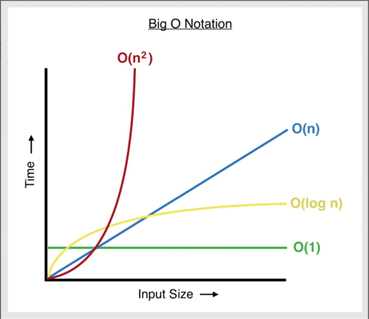
Complexity Comparison Between Typical Big Os
Let’s take an example. To solve the same problem, you have two functions:
f(n) =4n^2 +2n+4 and g(n) =4n+4
For f(n) =4n^2+2n+4
so here
f(1)=4+2+4
f(2)=16+4+4
f(3)=36+6+4
f(4)=64+8+4
As you can see here, the contribution of n^2 is a quadric function whose value will increase with the increase in the value of n. So when their value of n becomes very large, the contribution of n^2 will be 99% of the value on f(n).
So here, low-order terms can be ignored as they are relatively insignificant, as described above.
In this f(n), we can ignore 2n and 4 in comparison to n^2.
So,
n^2+2n+4 ——–>n^2. So here n^2 is highest rate of growth.
For g(n) =4n+4
so here
g(1)=4+4
g(2)=8+4
g(3)=12+4
g(4)=16+4
As you can see here, the contribution of n increases when we increase the value of n. So when the value of n becomes very large, the contribution of n will be 99% of the value of g(n). Therefore, we can ignore low-order terms as they are relatively insignificant. In this g(n), four and also four asconstant multipliers can also be ignored as it will have no effect as seen above so 4n+4 ——–>n.
We are not considering terms that are growing slowly and have not much effect in comparison to other terms and keep one which grows fastest.
Time Complexity:
Time Complexity is a way of representing or getting to know how the run-time of a function increases/decreases as the size of the input increases/decreases.
There are many types of time complexity, for example:
Linear Time —-> Already discussed in the above scenario where we helped my cousin from being embarrassed in front of his friends.
Constant Time —-> Here, the execution time for the function remains constant even though increasing the value of n at a very high rate.
Quadratic Time —-> Here, the execution time for functions increases in an exponential form on increasing the value of n.
If you don’t understand the meme, then you probably want to read about the very famous problem Travelling Salesman (Dynamic Programming).
Here are five Big O run times that you’ll encounter a lot, sorted from fastest to slowest:
O(log n), also known as log time. Example: Binary search.
O(n), also known as linear time. Example: Simple search.
O(n * log n). Example: A fast sorting algorithm, like quicksort.
O(n2). Example: A slow sorting algorithm, like selection sort.
O(n!). Example: A really slow algorithm, like a travelling salesperson.
Let’s understand the Big O Notation thoroughly by taking the C++ examples on common orders of growth, like,
Image Source: How To Calculate Time Complexity With Big O Notation | by Maxwell Harvey Croy | DataSeries | Medium
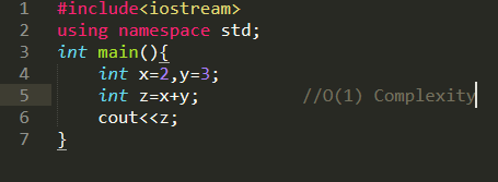
O(1) – Constant Time Algorithms
The O(1) is also called constant time, it will always execute at the same time regardless of the input size.
For example, if the input array could be 1 item or 100 items, this method required only one step. Note: O(1) is the best Time Complexity method.
2. O(LOG N) – Logarithmic Time Algorithms
In O(log n) function, the complexity increases as the size of the input increases.
Example: Binary Search.
3. O(N LOG N) – Linear Logarithmic Time Algorithms The O(n log n) function falls between the linear and quadratic function ( i.e, O(n) and Ο(n2). It is mainly used in sorting algorithms to get good Time complexity.
For example, Merge sort and quicksort.
For example, if the n is 4, then this algorithm will run 4 * log(8) = 4 * 3 = 12 times. Whether we have strict inequality or not in the for loop is irrelevant for the sake of a Big O Notation.
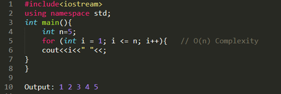
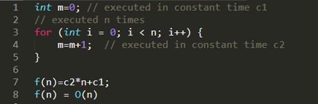
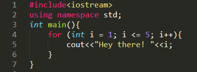
4. O(N) – Linear Time Algorithms The O(n) is also called linear time, it is in direct proportion to the number of inputs. For example, if the array has 6 items, it will print 6 times.
Note: In O(n), the number of elements increases, and the number of steps also increase.
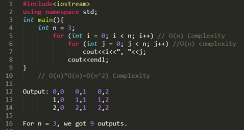
5. O(N2) – Polynomial-TimeAlgorithms The O(N2) is also called quadratic time. It is directly proportional to the square of the input size. For example, if the array has 3 items, it will print nine times.
Note: In O(N2), as the number of steps increases exponentially, the number of elements also increases. It is the worst-case Time Complexity method.
Note if we were to nest another for loop, this would become an O(n3) algorithm.
6. O(2N) – Exponential Time Algorithms
Algorithms with complexity O(2N) are called Exponential Time Algorithms.
These algorithms grow in proportion to some factor exponentiated by the input size.
For example, O(2N) algorithms double with every additional input. So, if n = 2, these algorithms will run four times; if n = 3, they will run eight times (kind of like the opposite of logarithmic time algorithms).
O(3N) algorithms triple with every additional input, O(kN) algorithms will get k times bigger with every additional input.
This algorithm will run 27 = 128 times.
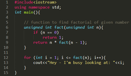
7. O(N!) – Factorial Time Algorithms
This class of algorithms has a run time proportional to the factorial of the input size.
A classic example of this is solving the travelling salesman problem using a brute-force approach to solve it.
where factorial(n) simply calculates n!. If n is 5, this algorithm will run 5! = 120 times.
Having trouble understanding the factorial code using recursion? Don’t worry. You can master the recursion from here. How to Master Recursion? – YouTube.
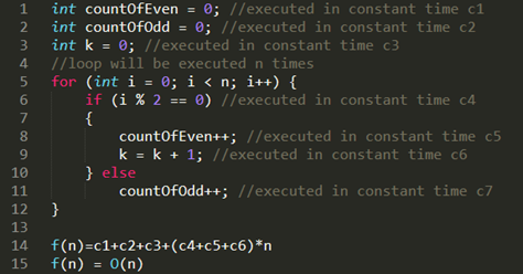
Rules of thumb for calculating the complexity of an algorithm: Simple programs can be analyzed using counting the number of loops or iterations.
The time complexity of a loop can be determined by the running time of statements inside the loop multiplied by the total number of iterations.
COMPLEXITY OF A NESTED LOOP: O(N^2)
It is the product of iterations of each loop.
COMPLEXITY OF IF AND ELSE BLOCK
When you have if and else statements, then time complexity is calculated with whichever of them is larger.
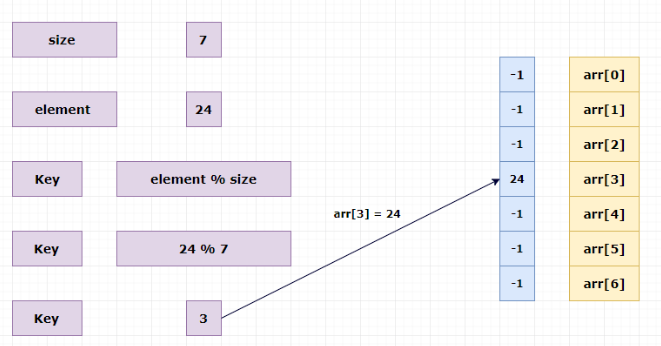
Example of Space Complexity
There could be times when you are required to optimize the space complexity of your algorithm, whether you’re doing competitive programming or working on real-time projects in development.
Remember that the factorial algorithm we discussed above it is using recursion, and always remember one thing recursion always makes stack, but it can also be optimised using dynamic programming where you can solve its space complexity.
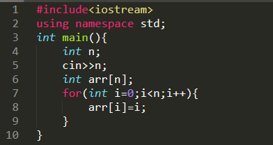
Now let’s have a look at a simple program and try to understand the space complexity.
Here I am not allocating any new variable, so the space complexity of my program is O(1). On the other hand, if I make another program like this.
Then you can see I have made an array of size n, so it’s causing the space complexity to be O(n).
Also, study Stack and Heap (memory management) so you can better understand the space complexity.
Big O Notation is used to describe the time complexity of an algorithm. We calculate the upper bound of algorithms runtime.
What is the best time complexity?
Best time complexity refers to the time taken by an algorithm. It refers to the lowest time required by an algorithm for a given input. In this, we calculate the lower bound of an algorithm.
What is the worst time complexity?
Best time complexity refers to the time taken by an algorithm. It refers to the maximum time required by an algorithm for a given input. In this, we calculate the upper bound of an algorithm.
What are the various types of Big O time complexity?
The five Bog O time complexity are O(log n), O(n), O(n * log n), O(n2), and O(n!).
What is the time complexity of Binary Search?
The time complexity of the binary search is O(log n). The best case is O(1) when the search input is in the first place.
Conclusion
Here are the main takeaways:
Algorithm speed isn’t measured in seconds but speed is measured in growth of the number of operations.
Instead, we talk about how quickly the run time of an algorithm increases/decreases as the size of the input increases/decreases.
Big O notation is helpful in expressing run time of algorithms.
O(log n) is faster than O(n), but it gets a lot faster as items in the list are huge/increasing drastically.


 9+ registered

