Breast Cancer Classification using KNN
I have downloaded the datasets from the Kaggle website and will work upon them by loading them to Google Colab.
First, import all the libraries that we need during the program.
import pandas as pd
import numpy as np
import matplotlib.pyplot as plt
import seaborn as sns
Now read the CSV file that contains breast-cancer datasets.
df = pd.read_csv("breast-cancer.csv")
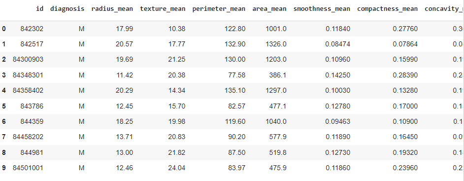
Once the dataset is in the data frame 'df,' let's print the first ten rows of the dataset.
df.head(10)
Output:

There are various features (columns) in the dataset; let's check them out.
df.shape
Output:

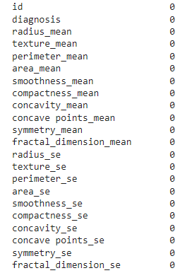
So, there are 569 rows and 33 columns in the dataset. Let’s count the number of empty (Nan, NAN, na) values in each column.
df.isna().sum()
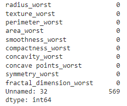
The above function gives the sum of all NaN values present in each of the features.
Output:


Column ‘Unnamed’ has 569 NaN values. So, we need to drop that column from the datasets.
Also, column ‘id’ doesn’t have any impact on predicting the output. So, we’ll drop this too.
df.drop(['Unnamed: 32','id'],axis='columns',inplace=True)
Now, let’s get the count of the number of Malignant(M) and Benign(B) cells in the diagnosis column.
df['diagnosis'].value_counts()
Output:

So, there are 357 Benign and 212 Malignant entries in the column ‘diagnosis’.
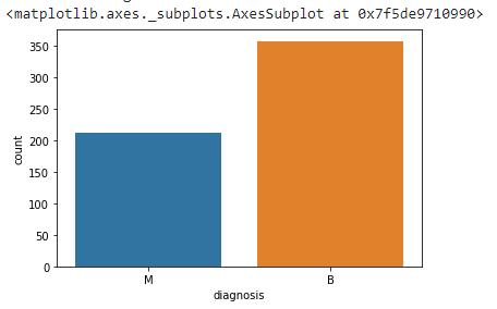
Let’s visualize the count of column ‘diagnosis’ using the seaborn library.
sns.countplot(df['diagnosis'])
Output:

It seems that Benign cases are more dominating than Malignant.
Now, I will encode the categorical values, i.e., Malignant(M) and Benign(B), with the help of a SKlearn library called LabelEncoder.
from sklearn.preprocessing import LabelEncoder
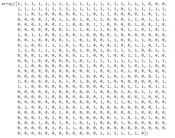
M is represented by the value 1, and B is represented by the value 0.

We can also get the correlation between the columns. The Correlation helps in finding whether one feature is associated with the other. Correlation coefficients range from [-1,1], endpoints inclusive. The Correlation coefficient of two numerical variables above +0.5 is a strong positive correlation, and the value below -0.5 is strongly negative.
The values in between these ranges are not that much correlated.
A strongly positive correlation between two variables denotes the direct relation between them. At the same time, a strongly negative depicts the inverse relationship between them. If two variables are not correlated, then one can't predict the other.
Let’s find the correlation table of the first five features.
df.iloc[:,0:5].corr()
Output:

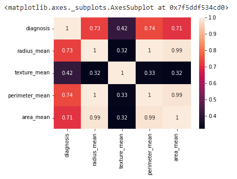
We can see that radius_mean, perimeter_mean, and area_mean have strong correlations with diagnosis. They are directly proportional to each other. In contrast, texture_mean has not had much correlation with the diagnosis.
Let’s visualize the correlations graphically.
sns.heatmap(df.iloc[:,0:5].corr(), annot=True)
Output:

We explored the data, manipulated it, and cleaned it. It’s time to create a model to detect Cancer cells.
Split the datasets into Independent (X) and Dependent (Y) datasets.
X = df.iloc[:,1:31].values
Y = df.iloc[:,0].values
The Target or dependent variable is the diagnosis, and the Independent variables are all the features except 'diagnosis.' X and Y are NumPy arrays.
Now, split the datasets into 80% training and 20% testing.
from sklearn.model_selection import train_test_split
X_train, X_test, Y_train, Y_test = train_test_split(X, Y, test_size = 0.2, random_state = 0)
Import KNN classifier from SKlearn module, and train the model using the fit function
from sklearn.neighbors import KNeighborsClassifier
clf = KNeighborsClassifier()
clf.fit(X_train, Y_train)
Let’s check the accuracy of the model.
clf.score(X_test, Y_test)
Output:

So, using the KNN classifier, the model predicts the 94% correct output.
Frequently Asked Questions
-
KNN does more computation on test time than train time; why?
=> There is no explicit training phase in KNN. It just takes data as input in its training phase. All the actual work. Ie. When the data is available, the computation of distances, comparisons, etc., is done in the testing phase.
-
What is the default value of K in KNN implemented in Sklearn?
=> 5
-
For k cross validation, smaller k value implies less variance?
=> True
-
Which of the techniques is generally used for feature selection in the case of KNN?
=> Back Elimination Algorithm
-
Which case do we need to handle separately to use KNN?
=> We need to handle the Categorical data, which has a feature, which can have values that don't have a natural ordering.
Key Takeaways
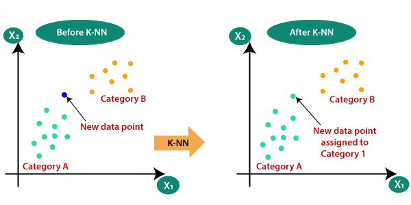
This comes to a brief Introduction and the detailed Implementation of Breast Cancer Classification Using KNN. For more knowledge about KNN, visit here.
( Must visit: NAIVE BAYES: IMPLEMENTATION FROM SCRATCH )
Thank You 😊😊
