Which optimizer is best for GAN?

Adam is the best optimizer till now for GAN implementation.

How many images does it take to train GAN?

A high-quality GAN is often trained using 50,000 to 100,000 training photos. However, in many circumstances, researchers simply do not have access to tens or hundreds of thousands of sample photos. Many GANs might struggle to provide realistic results with only a few thousand photos for training.

Do GANs need a lot of data?

GAN models are data-hungry, requiring massive amounts of varied and high-quality training samples to create high-fidelity natural pictures of various categories.

What is a discriminator in GAN?

In a GAN, the Discriminator is just a classifier. It attempts to distinguish between real data and data generated by the Generator. It might utilize any network architecture suitable for the sort of data it categorizes.

Building GAN - Implementation

Introduction

GANs (Generative Adversarial Networks) are a strong family of neural networks used for unsupervised learning. Ian J. Goodfellow created and launched it in 2014. GANs are composed of two competing neural network models that can analyze, capture, and duplicate the changes within a dataset.

Why was GAN developed?

Most standard neural networks can be readily misled into misclassifying items by introducing some noise into the original data. Surprisingly, the model's confidence in the incorrect prediction is higher after introducing noise than properly predicted. Such a problem is that most machine learning models learn on a little quantity of data, which is a significant disadvantage because it is prone to overfitting. Furthermore, the mapping between the input and the output is almost linear. Although the limits of separation between the various classes can be linear, they are made up of linearities, and even a little change in a point in the feature space can cause a large change in the feature space.

Also See, Resnet 50 Architecture

Working of GAN

GAN (Generative Adversarial Networks) can be broken down into three parts:

Generative: To learn a generative model that describes how data is generated in a probabilistic model.
Adversarial: The model is trained in an adversarial manner.
Networks: Use deep neural networks as the AI algorithms for training purposes.

GAN is made up of two parts: the Generator and the Discriminator. The Generator creates fake data samples to trick the Discriminator. On the other hand, the Discriminator attempts to distinguish between actual and fraudulent samples. Both the Discriminator and the Generator are Neural Networks, and they compete with each other throughout the training phase. The procedures are repeated multiple times, and with each iteration, the Generator and Discriminator grow better and better at their duties.

Let us implement a GAN using the cifar10 dataset.

Building GAN

Importing libraries

Let us import all the libraries that are required to implement the model.

from numpy import expand_dims, zeros, ones, vstack
from numpy.random import randn
from numpy.random import randint
from tensorflow.keras.datasets.cifar10 import load_data
from tensorflow.keras.optimizers import Adam
from tensorflow.keras.models import Sequential
from tensorflow.keras.layers import Dense, Reshape, Flatten, Conv2D, Conv2DTranspose, LeakyReLU, Dropout
from matplotlib import pyplot

You can also try this code with Online Python Compiler

Run Code

Discriminator Model

The first step towards implementing GAN is to implement a discriminator model, that takes input images from the dataset and outputs the prediction of the image, whether the image is real or fake.

The discriminator we are going to make will have three convolutional layers. Each layer will use a stride of 2×2 to downsample the input image. Also, we will use some good practices in making the model i.e., the use of LeakyReLU, Dropout, and Adam version of SGD.

# discriminator model
def discriminator(in_shape=(32,32,3)):
  model = Sequential()
  # normal
  model.add(Conv2D(64, (3,3), padding='same', input_shape=in_shape))
  model.add(LeakyReLU(alpha=0.2))
  # convolutional layer1
  model.add(Conv2D(128, (3,3), padding='same', strides=(2,2)))
  model.add(LeakyReLU(alpha=0.2))
  # convolutional layer2
  model.add(Conv2D(128, (3,3), padding='same', strides=(2,2)))
  model.add(LeakyReLU(alpha=0.2))
  # convolutional layer3
  model.add(Conv2D(256, (3,3), padding='same', strides=(2,2)))
  model.add(LeakyReLU(alpha=0.2))
  # flattening convolutional layer
  model.add(Flatten())
  model.add(Dropout(0.4))
  model.add(Dense(1, activation='sigmoid'))
  # compiling model
  opt = Adam(lr=0.0002, beta_1=0.5)
  model.compile(loss='binary_crossentropy', optimizer=opt, metrics=['accuracy'])
  return model

You can also try this code with Online Python Compiler

Run Code

Generator Model

The generator model creates new and fake objects. It accomplishes this by inputting a point from the latent space and producing a square color image.

The latent space is a 100-dimensional vector space with Gaussian-distributed values that can be freely defined. It has no meaning, but by randomly drawing points from this space and providing them to the generator model during training, the generator model will assign meaning to the latent points and, in turn, the latent space, until the latent vector space represents a compressed representation of the output space, CIFAR-10 images, that only the generator knows how to turn into plausible CIFAR-10 images at the end of training.

# generator model
def generator(latent_dim):
  model = Sequential()
  # foundation for 4x4 image
  n_nodes = 256 * 4 * 4
  model.add(Dense(n_nodes, input_dim=latent_dim))
  # using LeakyReLU activation
  model.add(LeakyReLU(alpha=0.2))
  model.add(Reshape((4, 4, 256)))
  # convolutional layer1
  model.add(Conv2DTranspose(128, (4,4), padding='same', strides=(2,2)))
  model.add(LeakyReLU(alpha=0.2))
  # convolutional layer2
  model.add(Conv2DTranspose(128, (4,4), padding='same', strides=(2,2)))
  model.add(LeakyReLU(alpha=0.2))
  # convolutional layer3
  model.add(Conv2DTranspose(128, (4,4), padding='same', strides=(2,2)))
  model.add(LeakyReLU(alpha=0.2))
  # output layer
  model.add(Conv2D(3, (3,3), padding='same', activation='tanh'))
  return model

You can also try this code with Online Python Compiler

Run Code

GAN

Here, we will combine both discriminator and generator model to make GAN.

def gan(g_model, d_model):
  # making weights in the discriminator non-trainable
  d_model.trainable = False
  # connecting discriminator and generator
  model = Sequential()
  # adding generator
  model.add(g_model)
  # adding discriminator
  model.add(d_model)
  # compiling model
  optzr = Adam(lr=0.0002, beta_1=0.5)
  model.compile(optimizer=optzr, loss='binary_crossentropy')
  return model

You can also try this code with Online Python Compiler

Run Code

Loading Dataset

Loading cifar10 dataset for GAN.

def load_real_samples():
  # load cifar10 dataset
  (trainX, _), (_, _) = load_data()
  # convert from unsigned ints to floats
  X = trainX.astype('float32')
  # scale from [0,255] to [-1,1]
  X = (X - 127.5) / 127.5
  return X

You can also try this code with Online Python Compiler

Run Code

Generating Latent Points, Fake Samples, Real Samples

# select real samples
def generate_real_samples(dataset, n_samples):
  # choosing random instances
  ri = randint(0, dataset.shape[0], n_samples)
  # retriving selected images
  X = dataset[ri]
  # generating 'real' class labels (1)
  y = ones((n_samples, 1))
  return X, y
 
# generating points in the latent space
def generate_latent_points(latent_dim, n_samples):
  # generating points
  x_input = randn(latent_dim * n_samples)
  # reshaping into a batch of inputs for the network
  x_input = x_input.reshape(n_samples, latent_dim)
  return x_input
 
# using the generator model to generate n fake examples, with class labels
def generate_fake_samples(g_model, latent_dim, n_samples):
  # generating points in latent space
  x_input = generate_latent_points(latent_dim, n_samples)
  # predicting outputs
  X = g_model.predict(x_input)
  # creating 'fake' class labels (0)
  y = zeros((n_samples, 1))
  return X, y

You can also try this code with Online Python Compiler

Run Code

Saving the Generated Image and Analyzing the Model

Saving the plot of image that are generated from generator model.

def save_plot(examples, epoch, n=7):
  # scale from [-1,1] to [0,1]
  examples = (examples + 1) / 2.0
  # plot images
  for i in range(n * n):
    # define subplot
    pyplot.subplot(n, n, 1 + i)
    # turn off axis
    pyplot.axis('off')
    # plot raw pixel data
    pyplot.imshow(examples[i])
  # save plot to file
  filename = 'generated_plot_e%03d.png' % (epoch+1)
  pyplot.savefig(filename)
  pyplot.close()
 
def summarize_performance(epoch, g_model, d_model, dataset, latent_dim, n_samples=150):
  # prepare real samples
  X_real, y_real = generate_real_samples(dataset, n_samples)
  # evaluate discriminator on real examples
  _, acc_real = d_model.evaluate(X_real, y_real, verbose=0)
  # prepare fake examples
  x_fake, y_fake = generate_fake_samples(g_model, latent_dim, n_samples)
  # evaluate discriminator on fake examples
  _, acc_fake = d_model.evaluate(x_fake, y_fake, verbose=0)
  # summarize discriminator performance
  print('>Accuracy real: %.0f%%, fake: %.0f%%' % (acc_real*100, acc_fake*100))
  # save plot
  save_plot(x_fake, epoch)
  # save the generator model tile file
  filename = 'generator_model_%03d.h5' % (epoch+1)
  g_model.save(filename)

You can also try this code with Online Python Compiler

Run Code

Training the GAN

Now we will train the GAN model that we created.

def train(g_model, d_model, gan_model, dataset, latent_dim, n_epochs=50, n_batch=128):
  bat_per_epo = int(dataset.shape[0] / n_batch)
  half_batch = int(n_batch / 2)
  # manually enumerate epochs
  for i in range(n_epochs):
    # enumerate batches over the training set
    for j in range(bat_per_epo):
      # get randomly selected 'real' samples
      X_real, y_real = generate_real_samples(dataset, half_batch)
      # update discriminator model weights
      d_loss1, _ = d_model.train_on_batch(X_real, y_real)
      # generate 'fake' examples
      X_fake, y_fake = generate_fake_samples(g_model, latent_dim, half_batch)
      # update discriminator model weights
      d_loss2, _ = d_model.train_on_batch(X_fake, y_fake)
      # prepare points in latent space as input for the generator
      X_gan = generate_latent_points(latent_dim, n_batch)
      # create inverted labels for the fake samples
      y_gan = ones((n_batch, 1))
      # update the generator via the discriminator's error
      g_loss = gan_model.train_on_batch(X_gan, y_gan)
      # summarize loss on this batch
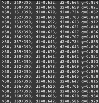
      print('>%d, %d/%d, d1=%.3f, d2=%.3f g=%.3f' %
        (i+1, j+1, bat_per_epo, d_loss1, d_loss2, g_loss))
    # evaluate the model performance, sometimes
    if (i+1) % 10 == 0:
      summarize_performance(i, g_model, d_model, dataset, latent_dim)

You can also try this code with Online Python Compiler

Run Code

Final Step

Lastly, we will call all the functions that we created.

# defining size of latent space 
latent_dim = 100
# calling discriminator function
d_model = discriminator()
# calling generator function
g_model = generator(latent_dim)
# calling gan function
gan_model = gan(g_model, d_model)
# load image data
dataset = load_real_samples()
# training the model
train(g_model, d_model, gan_model, dataset, latent_dim)

# plotting the generated images
def create_plot(examples, n):
  for i in range(n * n):
    pyplot.subplot(n, n, 1 + i)
    pyplot.axis('off')
    pyplot.imshow(examples[i, :, :])
  pyplot.show()

# loading the model
model = g_model
# generating images
latent_points = generate_latent_points(100, 100)
# generating images
X = model.predict(latent_points)
X = (X + 1) / 2.0
# plotting the result
create_plot(X, 10)

You can also try this code with Online Python Compiler

Run Code

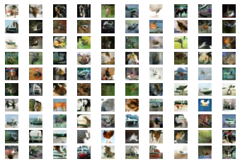
Output

The output will be huge, as shown below.

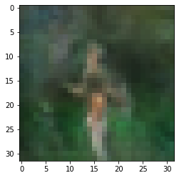
Generating an image for specific point in latent space.

vector = asarray([[0.75 for _ in range(100)]])
# generate image
X = model.predict(vector)
# scale from [-1,1] to [0,1]
X = (X + 1) / 2.0
# plot the result
pyplot.imshow(X[0, :, :])
pyplot.show()

You can also try this code with Online Python Compiler

Run Code

Training the above model takes nearly 2 hours in google colab GPU. Increase the number of epochs for better results (preferred 200+ epochs).

FAQs

Which optimizer is best for GAN?
Adam is the best optimizer till now for GAN implementation.
How many images does it take to train GAN?
A high-quality GAN is often trained using 50,000 to 100,000 training photos. However, in many circumstances, researchers simply do not have access to tens or hundreds of thousands of sample photos. Many GANs might struggle to provide realistic results with only a few thousand photos for training.
Do GANs need a lot of data?
GAN models are data-hungry, requiring massive amounts of varied and high-quality training samples to create high-fidelity natural pictures of various categories.
What is a discriminator in GAN?
In a GAN, the Discriminator is just a classifier. It attempts to distinguish between real data and data generated by the Generator. It might utilize any network architecture suitable for the sort of data it categorizes.

Key Takeaway

In this article, we have discussed the following topics:

Introduction to GAN
Working of GAN
GAN model

Want to learn more about Machine Learning? Here is an excellent course that can guide you in learning.

Also check out - Strong Number

Happy Coding!