Classic ConvNet Architectures

Classic ConvNet Architectures

There are various architectures in the field of Convolutional Networks that are most commonly used.

• LeNet: It is used to detect handwritten cheques by banks.
   
• AlexNet: It is used for any object-detection task.
   
• ZF Net: It is used in a diagnostic role.
   
• GoogLeNet: It is used for face detection and recognition.
   
• VGGNet: It is used for image recognition.
   
• ResNet: It is used to train intense neural networks.

We will explore each architecture in this section. But before we start we must know the important concepts that are used in almost every architecture. We will not go in-depth about these concepts but yes will take an overview of them to connect with the layers of architectures. 

Important Concepts to Understand CNN Architectures 

Here are some important concepts to understand:

Convolution and Filters

Convolution is a fundamental operation in CNNs. It involves sliding a small matrix called a filter or kernel over the input data, such as an image, and performing element-wise multiplications and summations.

This process extracts features by detecting patterns, edges, textures, or other visual attributes present in the data.

Convolutional Layers

Convolutional layers are the building blocks of CNN architectures. These layers consist of multiple filters applied in parallel, each producing a feature map. 

The filters in the early layers capture low-level features, while those in the deeper layers learn more complex and abstract features.

Pooling Layers

Pooling layers downsample the feature maps obtained from convolutional layers, reducing the spatial dimensions. Common pooling techniques include max pooling, where the maximum value in each pooling region is selected.

There also exists average pooling, which takes the average value from the matrix. 

Pooling helps to extract the most salient features and reduce computational complexity.

Activation Functions

Activation functions introduce non-linearity into CNN architectures, enabling them to learn complex relationships between input data and desired outputs. Popular activation functions include ReLU (Rectified Linear Unit), which sets negative values to zero, and sigmoid and tanh functions that squash values within a specific range.

Here is an example of ReLU: 

Fully Connected Layers

Fully connected layers, also known as dense layers, are traditionally found at the end of CNN architectures. These layers connect every neuron in one layer to every neuron in the subsequent layer. 

They capture high-level features and are responsible for producing the final outputs, such as classification probabilities.

For more information, you can read this article. 

Let us now move to discussing different types of Classic ConvNet Architectures. In this article, we have covered the overview of them and how they work. 

Let us start:

LeNet-5 Architecture

History : LeNet-5 was one of the first successful CNNs and laid the foundation for many subsequent advancements in computer vision tasks. It was developed by Yann LeCun and his colleagues in the late 1990s. It was specifically designed for handwritten digit recognition, but its principle influenced many machine learning models. 

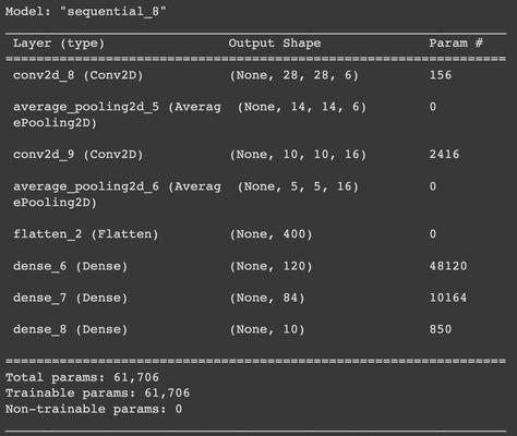
The LeNet-5 architecture consists of 7 layers:

1. Input layer: The input layer is a 32x32 grayscale image.
    
2. Convolutional layer 1: This layer has 6 feature maps, each of which is a 28x28x6 tensor. The kernel size is 5x5 and the stride is 1. Average pooling layer 1: This layer reduces the size of the feature maps by half, to 14x14x6. The kernel size is 2x2 and the stride is 2.
    
3. Convolutional layer 2: This layer has 16 feature maps, each of which is a 10x10x16 tensor. The kernel size is 5x5 and the stride is 1. Average pooling layer 2: This layer reduces the size of the feature maps by half, to 5x5x16. The kernel size is 2x2 and the stride is 2.
    
4. Flattening layer: This layer flattens the 5x5x16 tensor into a 400-dimensional vector.
    
5. Fully connected layer 1: This layer has 120 neurons.
    
6. Fully connected layer 2: This layer has 84 neurons.
    
7. Output layer: This layer has 10 neurons, one for each digit.

The LeNet-5 architecture is a simple and efficient architecture that has been used as a benchmark for many other CNN architectures. It is a good choice for image classification tasks that require high accuracy, such as handwritten digit recognition.

Here is the code by using Keras: 

from keras.models import Sequential
from keras.layers import Conv2D, AveragePooling2D, Flatten, Dense
model = keras.Sequential()

model.add(Conv2D(filters=6, kernel_size=(5, 5), activation='relu', input_shape=(32,32,1)))
model.add(AveragePooling2D(pool_size = (2,2), strides=2, padding='valid'))

model.add(Conv2D(filters=16, kernel_size=(5, 5), activation='relu'))
model.add(AveragePooling2D(pool_size = (2,2), strides=2, padding='valid'))

model.add(Flatten())

model.add(Dense(units=120, activation='relu'))

model.add(Dense(units=84, activation='relu'))

model.add(Dense(units=10, activation = 'softmax'))

Let us see its summary: 

model.summary()

Result:

Next, let us now discuss the AlexNet architecture: 

AlexNet Architecture  

History : AlexNet is a deep convolutional neural network (CNN) architecture that achieved remarkable success in the ImageNet Large-Scale Visual Recognition Challenge (ILSVRC) in 2012. It was developed by Alex Krizhevsky, Ilya Sutskever, and Geoffrey Hinton. Out of them, AlexNet played a pivotal role in popularizing deep learning and advancing computer vision tasks. 

It consists of multiple convolutional and fully connected layers and introduced several key concepts that are now widely used in CNN architectures.

• Input Layer: The network takes an input image of size 227x227 pixels with three color channels (RGB).
   
• Convolutional Layer 1: Applies 96 filters of size 11x11 pixels with a stride of 4 pixels. Introduces non-linearity through the ReLU activation function.
   
• Max Pooling Layer 1: Performs max pooling using a 3x3 window with a stride of 2 pixels. Reduces the spatial dimensions of the feature maps. Also, remember in max pooling layer, we don’t use any kernel, so it remains the same as before. In this case: it will be 96 only. 
   
• Convolutional Layer 2: Applies 256 filters of size 5x5 pixels. Introduces ReLU activation.
   
• Max Pooling Layer 2: Performs max pooling with a 3x3 window and a stride of 2 pixels.
   
• Convolutional Layer 3: Applies 384 filters of size 3x3 pixels. Introduces ReLU activation.
   
• Convolutional Layer 4: Applies 384 filters of size 3x3 pixels. Introduces ReLU activation.
   
• Convolutional Layer 5: Applies 256 filters of size 3x3 pixels. Introduces ReLU activation.
   
• Max Pooling Layer 3: Performs max pooling with a 3x3 window and a stride of 2 pixels.
   
• Flatten Layer: Flattens the output of the previous layer into a 1D vector.
   
• Fully Connected Layer 1: Contains 4096 neurons. Applies ReLU activation.
   
• Dropout Layer 1: Regularizes the network by randomly setting 50% of the neurons' outputs to zero during training.
   
• Fully Connected Layer 2: Contains 4096 neurons. Applies ReLU activation.
   
• Dropout Layer 2: Regularizes the network by randomly setting 50% of the neurons' outputs to zero during training.
   
• Fully Connected Layer 3 (Output Layer): Contains 1000 neurons, representing the 1000 classes in the ImageNet dataset. Uses softmax activation to produce class probabilities.

           Source: https://neurohive.io/

In the above diagram every step is explained. Now you must be wondering how the dimensions are being updated after every convolutional layer. 

So, there is a formula: ((n + 2p - f) / s ) + 1

where, n is the number of pixels,

p is the padding size,

f is the number of filters, 

And s is the number of strides used. 

If we take an example of the first convolutional layer ( Input Image): 

n = 227, p = 0 ( since we are not using padding ), f = 11 and s = 4. 

To calculate the next feature map: ( 227 + 2(0) - 11 ) / 4 = 216/4 = 54 + 1 = 55.  

For more understanding of AlexNet architecture, you can calculate the dimensions after every convolutional layer. 

One question may arise in your mind, why AlexNet if we already have LeNet-5 architecture. 

Because it introduces other concepts like: ReLu activation, Standardization ( Local Response Normalization ), Dropout and Enhanced Data ( Data Augmentation ). 
 

• ReLU activation is used after each convolutional layer to introduce non-linearity and facilitate learning complex patterns.
   
• Local Response Normalization (LRN) is applied after the first and second convolutional layers to enhance generalization.
   
• Dropout is employed after the first two fully connected layers to mitigate overfitting.
   
• Max pooling layers are utilized to reduce spatial dimensions and retain important features.
   
• The model is trained using stochastic gradient descent with momentum.
   
• Data augmentation techniques, such as random cropping and horizontal flipping, are applied to improve generalization.
   

Next up is ZF Net architecture: 

ZF Net Architecture 

History : The ZF Net architecture, also known as the Zeiler & Fergus Net, is a convolutional neural network (CNN) architecture proposed by Matthew D. Zeiler and Rob Fergus in 2013. It was designed to improve upon the performance of previous CNN models, particularly in the task of object recognition. The ZF Net architecture builds upon the concepts introduced by AlexNet and incorporates several modifications.
 

Below are the layers that are presented in ZF Net architecture: 
 

• The input layer accepts RGB images of size 227x227 pixels.
   
• The architecture includes several convolutional layers, gradually learning complex features. The first layer uses a 7x7 filter with a stride of 2 pixels, followed by subsequent layers using smaller filter sizes (5x5, 3x3, 3x3).
   
• ReLU activation is applied after each convolutional layer to introduce non-linearity.
   
• Local Response Normalization (LRN) is used to normalize responses across feature maps, enhancing generalization.
   
• Max pooling layers with a 3x3 window and a stride of 2 pixels reduce spatial dimensions and capture important features.
   
• Deconvolutional layers (upsampling) are introduced to increase spatial resolution and learn finer details. The deconvolutional layers in ZF Net play a crucial role in object localization, allowing the network to learn finer details and provide more accurate localization information. 
   
• The deconvolutional layers are concatenated with corresponding convolutional layers to combine high-resolution information with high-level features.
   
• Fully connected layers follow, with two layers consisting of 4096 neurons each. ReLU activation is applied after each fully connected layer.
   
• Dropout regularization is utilized after the first fully connected layer to mitigate overfitting.
   
• The final fully connected layer varies in the number of neurons based on the task, using softmax activation to produce class probabilities.

Source: medium.com

So, what’s the unique point here: Deconvolutional Layer. 

By introducing deconvolutional layers, ZF Net enables the network to capture and propagate more detailed spatial information throughout the architecture. This helps in localizing objects more accurately and improving performance on tasks that require precise spatial reasoning.

Next, let us now discuss the GoogleNet architecture: 

GoogleNet Architecture 

History : GoogleNet also known as inception-1 architecture developed by researchers at Google in 2014. It is a type of neural network designed to recognize and understand images. The key idea behind GoogleNet is the Inception module. This module allows the network to extract features from different sizes of input simultaneously, which helps capture a wide range of information.
 

Below are the layers present in GoogleNet architecture:

• Input Layer: The network takes an input image of variable size, typically resized to 224x224 pixels, with 3 color channels (RGB).
   
• Convolutional Layers: The initial layers are traditional convolutional layers with small filter sizes (3x3 and 5x5) and small strides. These layers extract basic features from the input image. 
   
• Inception Modules: The core building blocks of GoogleNet are the Inception modules. 
  
  
  • An Inception module performs feature extraction with filters of multiple sizes (1x1, 3x3, and 5x5) simultaneously. 
     
  • This allows the network to capture features at different spatial scales and encourages diverse and rich representations. 
     
  • Inception modules also include 1x1 convolutions, which help reduce the computational complexity by reducing the number of input channels before applying larger filters.
     
• Max Pooling Layers: Max pooling layers are throughout the architecture to reduce the spatial dimensions of the feature maps and capture the most salient features. In a nutshell, it is used to reduce the size of the input image. 
   
• Auxiliary Classifiers: GoogleNet includes auxiliary classifiers at intermediate stages of the network to combat the vanishing gradient problem. These auxiliary classifiers are additional branches that have their own smaller softmax layers and are trained with the main loss function. They encourage intermediate feature layers to contribute to the overall loss, aiding in gradient flow and improving training.
   
• Average Pooling and Fully Connected Layers: Towards the end of the architecture, average pooling is applied to further reduce the spatial dimensions. This is followed by fully connected layers with dropout regularization to learn high-level representations and mitigate overfitting.
   
• Output Layer: The final fully connected layer has a variable number of neurons based on the task at hand. For example, in object recognition tasks, the number of neurons corresponds to the number of classes. Softmax activation is typically applied to produce class probabilities. 
   

In the below architecture, every box represents a layer,

• Blue Box - Convolutional Layer
• Green Box - Feature Concatenation
• Red Box - MaxPool Layer
• Yellow Box - Softmax Layer

Next up is VGGNet architecture: 

VGGNet Architecture 

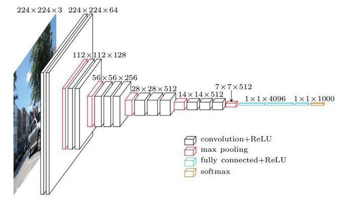
History : The VGGNet architecture, also known as the OxfordNet, is a convolutional neural network (CNN) architecture developed by Simonyan and Zisserman in 2014. It is named after the Visual Geometry Group (VGG) at the University of Oxford. VGGNet is well-known for its depth and simplicity, consisting of multiple layers with small convolutional filters.
 

Let us discuss its layers: 
 

• Input Layer: The network takes an input image of size 224x224 pixels with 3 color channels (RGB). 
   
• Convolutional Layers: The architecture uses 3x3 convolutional filters with a stride of 1 pixel and a padding of 1 pixel. Whenever we want the size to remain the same as before, padding is used to accomplish the same. 
   
• Activation Function: The ReLU (Rectified Linear Unit) activation function is applied after each convolutional layer to introduce non-linearity, helping the network learn complex patterns.
   
• Max Pooling Layers: Max pooling layers with a 2x2 window and a stride of 2 pixels are used throughout the architecture. 
   
• Fully Connected Layers: VGGNet typically includes multiple fully connected layers with a large number of neurons (e.g., 4096 neurons).
   
• Dropout: To mitigate overfitting, dropout regularization is applied after the fully connected layers. 
   
• Output Layer: The final fully connected layer has a variable number of neurons based on the task at hand. For example, in object recognition tasks, the number of neurons corresponds to the number of classes. Softmax activation is commonly used to produce class probabilities.

Source: Research Gate 

Next, let us now discuss the ResNet architecture: 

ResNet Architecture 

History : ResNet is the last architecture that was developed by researchers at Microsoft in 2015 to address the challenge of training very deep networks without the problem of vanishing gradients, which can hinder learning.

The key idea behind ResNet is the introduction of "skip connections" or "shortcut connections." These connections allow the network to skip over some layers and directly pass information to deeper layers.

Below is the flow of the ResNet architecture: 

• Input Layer: The network takes an input image of size 224x224 pixels with 3 color channels (RGB). 
   
• Convolutional Layers: The initial layers of ResNet consist of convolutional layers that perform feature extraction from the input image. 
   
• Residual Blocks [IMP]: The key innovation of ResNet lies in the residual blocks. Each residual block contains multiple convolutional layers, and within each block, there is a shortcut or skip connection. This connection allows the input to be directly added to the output of the block, creating a "residual" that represents the difference between the input and output.
   
• Identity Mapping: This concept is known as identity mapping, where the network is encouraged to learn only the residual information required to improve the predictions.
   
• Bottleneck Structure: ResNet commonly uses a bottleneck structure within the residual blocks. It involves reducing the dimensionality of the input with a 1x1 convolutional layer, followed by a 3x3 convolutional layer, and then expanding the dimensionality again with another 1x1 convolutional layer. This structure helps reduce computational complexity while maintaining representational power.
   
• Shortcut Connections: The shortcut connections in ResNet allow the gradients to flow more easily during backpropagation. 
   
• Global Average Pooling: Instead of using fully connected layers at the end of the network, ResNet typically applies global average pooling. This pooling operation computes the average value of each feature map across its spatial dimensions, resulting in a one-dimensional vector. It helps reduce overfitting and parameter count while preserving important information.
   
• Output Layer: The final layer of ResNet is a fully connected layer with softmax activation, which produces the predicted probabilities for different classes in a classification task.

Source: StackExchange

Frequently Asked Questions

What is the difference between neural networks and convolution neural networks?

CNN has a different design than regular neural networks. Neural networks transform an input by putting it through a series of hidden layers. In CNN, every layer comprises a set of neurons where each layer is fully connected to all neurons in the previous layer. 

Why is CNN used for image classification?

CNN is used for image classification and recognition because of its high accuracy. The CNN follows a hierarchical model that builds a network, like a funnel, and finally gives out a fully-connected layer where all the neurons are connected, and the output is processed. 

Why is CNN preferred over other algorithms?

The main reason that CNN is preferred over other algorithms is that it automatically detects the necessary features without any human supervision. For example, if it is given many pictures of cats and dogs, it learns distinctive features for each class by itself. CNN is also computationally efficient.

What is the vanishing gradient problem?

In the deep neural networks, as we propagate back to the starting or initial layers from the last layers, the gradient tends to vanish; it is known as the vanishing gradient problem.

Conclusion

To conclude the discussion, CNN is the most commonly used algorithm for image classification; it detects the essential features in an image without any human intervention. This article gave a detailed description of Convolution Neural Networks and its architectures. 

Check out this link if you are a Machine Learning enthusiast or want to brush up your knowledge with ML blogs.

You can also check out our other blogs, 

• Keras models
   
• Addressing Modes of 8086
   

Refer to our guided paths on Coding Ninjas Studio to learn more about DSA, Competitive Programming, JavaScript, System Design, etc. Enrol in our courses and refer to the mock test and problems available. Take a look at the interview experiences and interview bundle for placement preparations.

Happy Learning Ninja!