Introduction
Supervised Machine learning algorithms are employed to tackle two kinds of tasks - Classification and Regression.
It’s fundamental for data scientists to clearly differentiate between classification and regression tasks to employ correct techniques to solve a certain problem. Regression problems have continuous output variables, that is, the outputs aren’t bound within a set of absolute values.
Suppose a model predicts house prices in Delhi in a specific month. Now, these house prices could take any value. It could be said that the output variable, in this case, is continuous, and hence this is a regression task.
On the other hand, classification tasks have categorical(or discrete) target variables. Like a model that predicts if a person would turn out to be a loan defaulter or not, based on which a bank can decide if they want to sanction their loan.
Both the tasks have specific algorithms which may or may not be suited for the other.
Regression
As discussed earlier, regression tasks have continuous output variables. Regression analysis is often required in the domain of finance and investing in finding the relationship between independent variables and the dependent variable. Some of the popular regression algorithms are discussed below:-
Linear Regression
Linear regression tries to find a linear relationship between the dependent and independent variables. The algorithm tries to find the best fit line for the data points on the X-Y plane. It is given by the formula:-
y=a0x+a1
Where,
y = dependent variable
x = independent variable
a0 = linear regression coefficient (slope)
a1 = y intercept
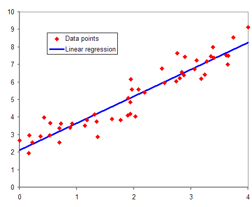
Source - link
Linear regression is of two types -
- Simple Linear regression:- One independent and one dependent variable (x , y).
- Multiple linear regression:- Several independent variables for one dependent variable ( (x0,x1,x2…..xn) , y).
To check how well the line depicts the relationship between the data points, a cost function is used.
Mean Squared Error (MSE) = 1/N ∑(actual-forecast)2
N = total number of values
actual = actual value (as given in (x,y) coordinates)
forecast = predicted value (as predicted by the function a1.X + a0 )
The cost function checks for which values of ao and a1 is the function most accurate.
Pros
- Easy to implement.
- Less complex than other regression techniques.
Cons
- The accuracy of the algorithm is vulnerable to outliers.
- Real-world problems aren’t usually simple enough to form a linear relationship.
Support Vector Regression(SVR)
You might have heard about Support Vector Machines(SVM). It’s a popular algorithm that is widely used for classification tasks. SVR uses a similar concept but to predict real values. The data points on the X-Y plane are segregated via hyperplanes. The dimensions can be increased in case this segregation is not possible.
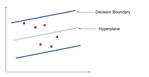
Hyperplane is our best fit line with maximum data points. Consider Decision boundaries to be at a distance of ‘s’ from the hyperplane. Our primary task is to decide this distance so that points closest to the hyperplane are within the boundary lines. Hence we are going to consider only those points that are within the boundary line and have the least error.
Pros
- SVR can accommodate outliers.
- They have excellent generalisation capabilities.
Cons
- Not well suited for large datasets.
- Not well suited for datasets with a lot of noise.
LASSO Regression
LASSO is an acronym for Least Absolute Selection Shrinkage Operator. Shrinkage here refers to shrinkage of parameters
LASSO applies constraints on attributes that cause regression coefficients of some variables to tend to zero.
Variables whose coefficients are shrunk to zero are neglected from the model. This basically means that these features are not important in deciding the best fit line of our model. So essentially it makes a feature selection.
Let us understand with an example.
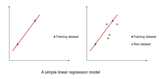
In the above figure, we took a small dataset to train a simple linear regression model.
The best fit line had a very low bias. However, the results were underwhelming when the model was tested on the test dataset. There was a very high variance. This is the case of overfitting when the model has a low bias(the line fits training data very well) and high variance(the line doesn’t fit the testing data very well). This is owing to the cost function used in the simple linear regression.
Mean Squared Error (MSE) = 1/N ∑(actual-forecast)2
The cost function minimised the sum of residuals. But it leads to the case of overfitting.
LASSO regression tweaks that cost function a bit to tackle this problem of overfitting.
The cost function in LASSO regression is :-
Cost function = 1/N ∑(actual-forecast)2 + λ |slope|
Where λ can take any value between 0 and infinity. The value is selected using cross-validation.
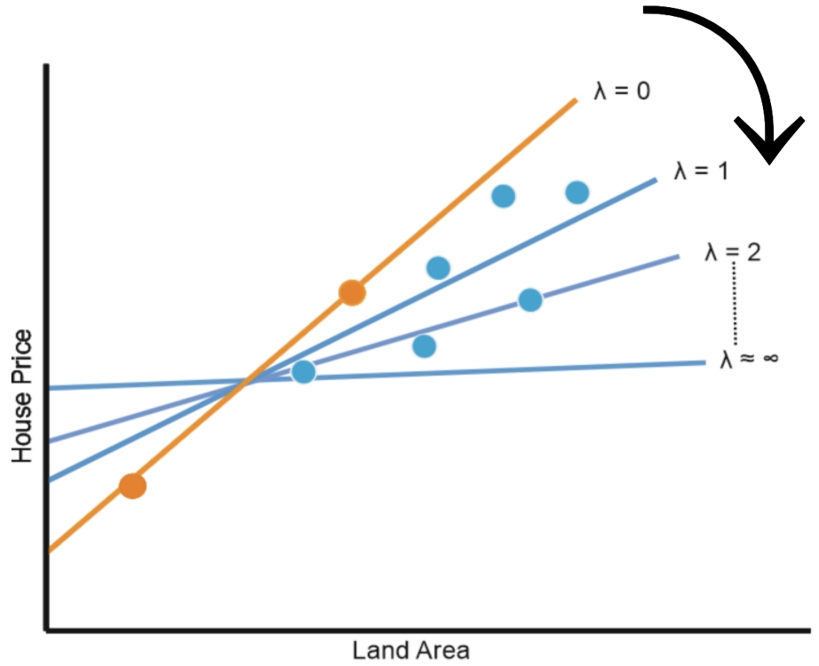
Source- Link
The LASSO regression cost function penalises higher-order slopes. These higher-order slopes generally lead to overfitting. We need to keep in mind that our model needs to be a general model which makes uniform predictions throughout our training and testing data. So to reduce overfitting, we make a trade-off between bias and variance. In the case of overfitting, the bias was close to zero but variance was huge. The additional term in the cost function balances bias and variance, hence generalising our model.
Pros
- It helps overcome the problem of overfitting.
Cons
- Selected parameters can be highly biased.
Ridge Regression
It is another regularisation technique, not much different from LASSO regression.
They differ just slightly in their cost function.
Cost function = 1/N ∑(actual-forecast)2 + λ (slope)2
Ridge regression also addresses the problem of overfitting in linear regression by making the bias-variance tradeoff, Just like LASSO regression. And the value of λ can be between 0 to infinity and is chosen by cross-validation, just like LASSO regression.
However, they differ in shrinkage of the coefficients. In LASSO regression, the shrinkage of any coefficient could go all the way down to zero. But in Ridge regression, the shrinkage never goes all the way down to zero, no matter how high the value of the coefficient of penalty (λ) is.
So unlike LASSO regression where we were essentially doing feature selection by shrinking the values of some coefficients all the way down to zero, in ridge regression that is not the case. But it’s intuitive to learn that the smaller the value of the coefficient becomes, the lesser it will make in choosing in the final model.


