Cloud Profiler

Profiling Applications

Continuous profiling of applications in production is an effective way to find where resources like CPU utilisation and memory are consumed. Cloud Profiler supports profiling based on the language in which a program is written. We use a profiling agent to instrument an application to capture profile data. The profiling agent collects the data, which can be viewed on the console interface in Google Cloud. It is installed on the virtual machines where the application runs. The agent comes as a library that is attached to the application at runtime.

Java Applications

The profile types supported for Java are CPU time, Heap and Wall time. 

Supported language versions are OpenJDK and Oracle JDK for Java 8, 11 or later.

Supported environments include Compute Engine, GKE, App Engine Flexible and Standard Environment, Dataproc and other external environments.

An underlying Profiler API is necessary to use a Profile Agent. We can enable this API by running the following command on gcloud CLI.

gcloud services enable cloudprofiler.googleapis.com.

The Profiler Agent can be installed according to the application's environment. To get a list of all the agent versions, run the command.

gsutil ls gs://cloud-profiler/java/cloud-profiler-*

The next step is to load the agent. Run the Java application and specify the agent-configuration options. To configure the profiling agent, insert an -agent path tag while starting the application. 

-agentpath:INSTALL_DIR/profiler_java_agent.so=OPTION1,OPTION2,OPTION3

We specify a service-name argument and an optional service-version argument to configure it. The service name allows the Profiler to collect profiling data for all replicas of that service. 

External Applications

Although the application and the Cloud Profiler agent run outside Google Cloud, the Cloud Profiler interface is required to analyse the profiling data. This requires a Google Cloud Project.

Step 1: Create a Google Cloud project and enable the Profiler API.

Step 2: Obtain the profiling agent's credentials when uploading profiles.

Step 3: Configure and allow the agent to use the credentials and the ID of the Google Cloud project.

We can use a service account to enable the agent. The account must have the roles/cloudprofiler.agent role to write profiling data. To use application default credentials, run the command.

-agentpath:INSTALL_DIR/profiler_java_agent.so=OPTION1,OPTION2,OPTION3

Link the agent to the Cloud Project. The profiling agent must be configured to specify the ID of the Google Cloud project to upload profiles. This requires an additional Java agent configuration flag, cprof_project_id, on Java invocation.

-cprof_project_id=PROJECT_ID

Measure App Performance

Calculating the performance of production systems is tough and complex. Test environments usually fail to replicate the pressures on a production system. Using Cloud Profiler greatly reduces the complexity of this task.

Let’s consider a Go program that creates a CPU-intensive workload to provide data to the profiler.

git clone https://github.com/GoogleCloudPlatform/golang-samples.git
cd golang-samples/profiler/profiler_quickstart

Step 1: Go to the directory that contains the code. Start the program and let it run.

go run main.go

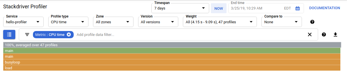
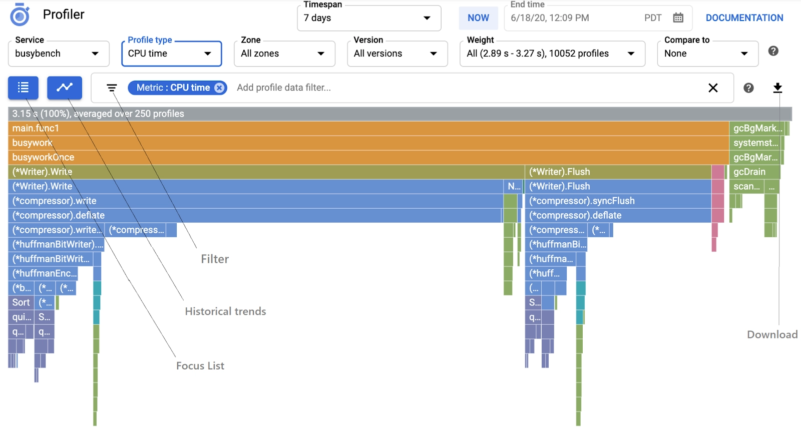
The program is designed to load the CPU as it runs. It is configured to use the Profiler to collect profiling data and periodically saves it. After a few minutes, we receive an indication that the profiler has started. In the profiler Interface, we can observe an array of controls and a flame graph for exploring the profiling data.
 

• The grey frame represents the entire executable. This accounts for 100% of the consumed resources.
   
• The green main frame represents the Go runtime.
   
• The orange main frame is the main routine of the sample program.
   
• The orange busyloop frame is called from the sample's main.
   
• The orange main.load frame is called from the sample's main.

Flame graphs

They help visualise hierarchical data and stack traces of profiled software so that the most frequent code paths can be identified quickly and accurately. Each rectangle represents a stack frame. The wider a frame is, the more often it was present in the stacks. Flame charts put the passage of time on the x-axis. This means that time-based patterns can be studied using flame graphs. Flame graphs efficiently use screen space by representing much information in a compact and readable format.

The following diagram shows how a  tree can be converted into a flame graph. Each tree node is represented with a frame.

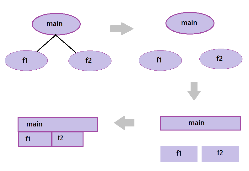
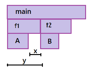
The frame width is a relative measure of that function's total CPU time. ‘Y’ represents the total CPU usage of function f1. The empty space below a frame is the relative measure of the self CPU time for the function in the frame. ‘X’ represents the self CPU usage of f1.

Focusing Flame graphs

The focus filter option present in the Profiler interface can be used to select functions. The flame graph displays the code paths specific to that function. A focused graph helps analyse the aggregate resource consumption of a given function called from multiple places. It can also analyse the proportion of time spent for different callers of the function. The graph built by the Focus filter effectively creates two flame graphs for a particular function and joins them together. The graph includes a separate frame for a focus function called Sort. It is a highlighted and full-width frame. The bottom half of the Sort frame assumes the starting point of a standard flame graph and shows all of its callees. The top half of the graph shows the callers of Sort with the callees hidden.

Selecting a frame in a focused graph redraws the flame graph displaying the frame's call stack in more detail. Users can set focus filters by using the graph, the focus list or the filter bar present in the interface. The focus filter can be removed by clicking Close on the filter.

Comparing Profiles

Cloud Profiler allows users to visually compare two profiles of the same type from the same service in a project. Profiles may differ by ending times, zones, service versions or weight.

We specify the parameters for an original profile and a compared profile to set up a comparison. The comparison type is set from the  Compare To menu. Fields like Timespan, End time, Profile type and service apply to the profiles set for comparison.

A comparison graph differs from the standard flame graph in terms of colours, block size and metric information. The colours in a comparison graph represent the difference between the total metric consumption of the function in the original and compared profile. Significant differences in consumption values between the two profiles display more saturated colours. The size of the function blocks indicates the relative average consumption of the metric being analysed. We can turn off comparison mode by setting the value of Compare to None.

View historical trends

The Cloud Profiler’s history view displays data for the most recent 30 days. Each line in a history chart shows a function's resource usage history. The Value type menu can display profile data as a percentage of the resource usage for all functions or as the absolute value in the metric's units. The Show up to menu allows users to configure the maximum number of functions to display. By default, it is set to 5 functions.

The chart title indicates if the chart shows self-usage or the total usage. It also identifies the resource being displayed. The chart legend lists the names of the functions on display.

Frequently Asked Questions

What are some of the errors that occur while using a Python profiling agent?

The NotImplementedError exception is thrown during the execution of the start function as the application runs in a non-Linux environment. The ValueError exception is thrown when the function's variables are invalid or can not be determined.

What roles and permissions can be set to access the profiling activities in Google Cloud?

Identity Access Management provides separate permission to create, list and modify profiles. Two different roles can be assigned to users, groups, and service accounts. The roles/cloudprofiler.agent for a Profiler agent and roles/cloudprofiler.user for a Profiler user.

How to set the range of time for which the profiling data is displayed?

The Timespan menu, the Now button, and the End time menu can be used to assign a time range. By default, Timespan is set to seven days, and End time contains the time when Profiler started and cannot be modified.

Conclusion

This blog discusses Cloud Profiler on GCP in detail. It describes the Profiler interface along with flame graphs. It also explains how to Profile applications and measure App Performance using Cloud Profiler.

Check out our articles on Cloud Logging in GCP, Monitoring Agent and Identity Access Management. Explore our Library on Coding Ninjas Studio to gain knowledge on Data Structures and Algorithms, Machine Learning, Deep Learning, Cloud Computing and many more! Test your coding skills by solving our test series and participating in the contests hosted on Coding Ninjas Studio! 

Looking for questions from tech giants like Amazon, Microsoft, Uber, etc.? Look at the problems, interview experiences, and interview bundle for placement preparations. Upvote our blogs if you find them insightful and engaging! Happy Coding!