Introduction
Support Vector Machines are machine learning model used for classification and regression analysis. SVM is basically the representation of examples as the points in a graph such that representation of separate category is divided by a wide gap that gap is as wide as possible.
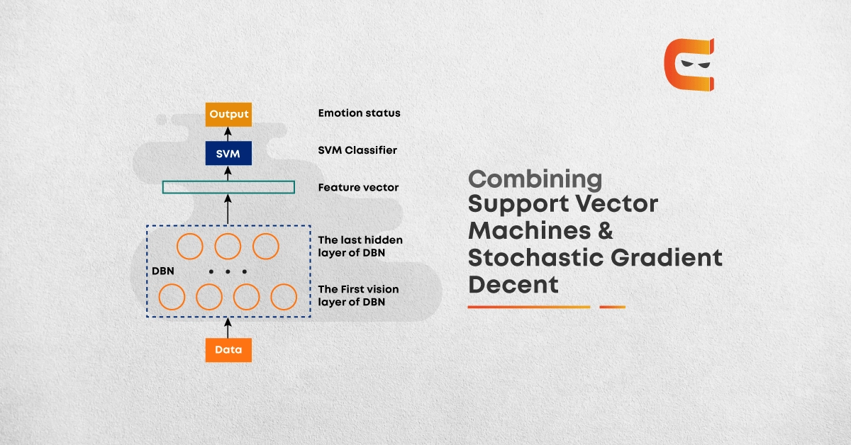
A new example is presented in that graphical points and is clearly mapped with the category by the distance of the point form the divided category. They are not only used for linear classification but also non-linear classification using kernel trick.
Hyperlane

SVM makes a hyperplane which creates a gap between the categorized data points. Finds an optimal hyperplane, that best separates our data so that the distance from nearest points in space to itself (also called margin) is maximised. A good separation is achieved by the hyperplane that has the largest distance to the nearest training-data point of any class (so-called functional margin), since in general the larger the margin, the lower the generalisation error of the classifier.
The hyperplanes in the higher-dimensional space are defined as the set of points whose dot product with a vector in that space is constant, where such a set of vectors is an orthogonal (and thus minimal) set of vectors that defines a hyperplane. A hyperplane is a plane of n-1 dimensions in n-dimensional feature space, that separates the two classes. For a 2D feature space, it would be a line and for a 3D Feature space, it would be plane and so on.
A hyperplane is able to separate classes if for all points:
- w x + b > 0 (For data points in class 1)
- w x + b < 0 (For data points in class 0)
This means the of all the point from class 1 the answer to the equation should be greater than 0 and for the other class as class 0 referred here should be less than 0.
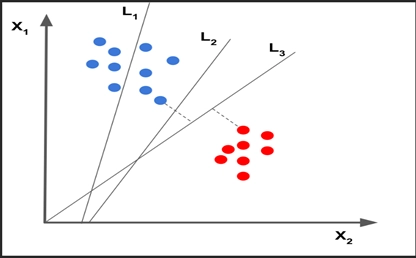
Maximum Margin Hyperplane: An optimal hyperplane best separates our data so that the distance/margin from nearest points (called Support Vectors) in space to itself is maximised is called Maximum Margin Hyperplane. These nearest points are called Support Vectors.

Applications: SVM’s because of the linear and non-linear classification they are used widely below are some real-world applications that are widely popular. They are not only can make reliable prediction but also can reduce redundant information.
- Handwriting recognition – We use SVMs to recognise handwritten characters used widely.
- Protein fold and remote homology detection – Apply SVM algorithms for protein remote homology detection.
- Face detection – SVMc classify parts of the image as a face and non-face and create a square boundary around the face.
- Text and hypertext categorisation – SVMs allow Text and hypertext categorisation for both inductive and transudative models. They use training data to classify documents into different categories. It categorizes on the basis of the score generated and then compares with the threshold value.
- Classification of images – Use of SVMs provides better search accuracy for image classification. It provides better accuracy in comparison to the traditional query-based searching techniques.
Stochastic Gradient Descent
The word ‘stochastic‘ means a system or a process that is linked with a random probability. Hence, in Stochastic Gradient Descent, a few samples are selected randomly instead of the whole data set for each iteration. In Gradient Descent, there is a term called “batch” which denotes the total number of samples from a dataset that is used for calculating the gradient for each iteration. In typical Gradient Descent optimisation, like Batch Gradient Descent, the batch is taken to be the whole dataset. Although, using the whole dataset is really useful for getting to the minima in a less noisy and less random manner, but the problem arises when our datasets get big.
Suppose, you have a million samples in your dataset, so if you use a typical Gradient Descent optimisation technique, you will have to use all of the one million samples for completing one iteration while performing the Gradient Descent, and it has to be done for every iteration until the minima are reached. Hence, it becomes computationally very expensive to perform. So, in SGD, we find out the gradient of the cost function of a single example at each iteration instead of the sum of the gradient of the cost function of all the examples.
If we implement SGD from basic using the basic scientific libraries in deep learning, we require 3 for-loop in total:
- Over the number of iterations
- Over the m training examples
- Over the layers (to update all parameters, from (W^([1]), b^([1])) to (W^([L]), b^([L])))
Here:
W^([1]): weight of first layer
W^([L]): weight of Lth layer
b^([1]): bias of 1st layer
b^([L]): bias of Lth layer
Comparing SGD with Gradient Descent: In Stochastic Gradient Descent, you use only 1 training example before updating the gradients. When the training set is large, SGD can be faster. But the parameters will “oscillate” toward the minimum rather than converge smoothly as in Gradient Descent. By the below diagram you can easily see the difference:

Comparing SGD with Mini-Batch Gradient Descent: In practice, you’ll often get faster results if you do not use neither the whole training set, nor only one training example, to perform each update. Mini-batch gradient descent uses an intermediate number of examples for each step. With mini-batch gradient descent, you loop over the mini-batches instead of looping over individual training examples.

SVM Implementation using Pegasos
Pegasos performs stochastic gradient descent on the primal objective with a carefully chosen stepwise.
Paper – Pegasos: Primal Estimated sub-Gradient Solver for SVM. The final SVM Objective we derived was as follows:

Here is the python implementation of SVM using Pegasos with Stochastic Gradient Descent. The Code below was implemented in Jupyter notebook so as we can see step by step implementation and visualisation of the code.
from matplotlib import pyplot as plt
from sklearn.datasets import make_classification

X, Y = make_classification(n_classes=2, n_samples=400, n_clusters_per_class=1, random_state=3, n_features=2, n_informative=2, n_redundant=0)

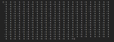
Convert our Y-Labels into {1,-1}

Y[Y==0] = -1 #Broadcasting
print(Y)
#Output
plt.scatter(X[:,0], X[:,1], c=Y)
plt.show()
#Output
import numpy as np
class SVM:
def init(self, C=1.0):
	self.C = C
	self.W = 0
	self.b = 0
def hingeLoss(self, W, b, X, Y):
	loss = 0.0
	loss += .5*np.dot(W, W.T)
	m = X.shape[0]
for i in range(m):
	ti = Y[i] * (np.dot(W, X[i].T) + b)
	loss += self.C *max(0, (1-ti))
return loss[0][0]
def fit(self, X, Y, batch_size=100, learning_rate=0.001, maxItr=300):
	no_of_features = X.shape[1]
	no_of_samples = X.shape[0]
	n = learning_rate
	c = self.C

# Init the model parameters

W = np.zeros((1, no_of_features))
bias = 0

# Initial Loss
# Training from here…
# Weight and Bias update rule that we discussed!

losses = []
for i in range(maxItr):
# Training Loop
	l = self.hingeLoss(W, bias, X, Y)
	losses. append(l)
	ids = np.arange(no_of_samples)
	np.random.shuffle(ids)
# Batch Gradient Descent(Paper) with random shuffling
for batch_start in range(0, no_of_samples, batch_size):
# Assume 0 gradient for the batch
	gradw = 0
	gradb = 0
# Iterate over all examples in the mini batch
for j in range(batch_start, batch_start + batch_size):
	if j < no_of_samples: i = ids[j] ti = Y[i] * (np.dot(W, X[i].T) + bias) if ti > 1:
		gradw += 0
		gradb += 0
	else:
		gradw += c * Y[i] * X[i]
		gradb += c * Y[i]
# Gradient for the batch is ready! Update W, B
	W = W – nW + ngradw
	bias = bias + n*gradb
	self.W = W
    self.b = bias
    return W, bias, losses
	mySVM = SVM(C=1000)
	W, b, losses = mySVM.fit(X, Y, maxItr=100)
	print(losses[0])
	print(losses[-1])
#Output

plt.plot(losses)
plt.show()
#Ouput

W, B = mySVM.W, mySVM.b
print(W, B)
#Output

def plotHyperplane(w1, w2, b):
	plt.figure(figsize=(12, 12))
	x_1 = np.linspace(-2, 4, 10)
	x_2 = -(w1x_1+b)/w2 # WT + B = 0 x_p = -(w1x_1+b+1)/w2 # WT + B = -1
	x_n = -(w1*x_1+b-1)/w2 # WT + B = +1

plt.plot(x_1, x_2, label=”Hyperplane WX+B=0″)
plt.plot(x_1, x_p, label=”+ve Hyperplane WX+B=1″)
plt.plot(x_1, x_n, label=”-ve Hyperplane WX+B=-1″)
plt.legend()
plt.scatter(X[:,0], X[:,1], c=Y)
plt.show()
plotHyperplane(W[0,0], W[0,1], B)
#Ouput
# Visualising Support Vectors, Positive and Negative Hyperplanes
# Effect the changing ‘C’ – Penalty Constant
plotHyperplane(W[0,0],W[0,1],B)
#Output
Frequently Asked Questions
Is SVM affected by feature scaling?
Yes, SVMs are sensitive to feature scaling because they use input data to find the margins around hyperplanes and become biassed for high-valued variance.
Should data be scaled before SVM?
When performing linear SVM classification, it is frequently useful to normalise the training data, for example, by subtracting the mean and dividing by the standard deviation, and then scale the test data with the mean and standard deviation of the training data.
In SVM, what is the maximum margin hyperplane?
The margin is the distance between the line and the nearest data points. The line with the greatest margin is the best or optimal line that can separate the two classes.


