Confusion Matrix with Tensorboard

Introduction

A confusion matrix is also known as an error matrix. It is in the form of a table that helps us to visualize the performance of the algorithm. In other words, we can say a confusion matrix is a plot of predicted vs. real classes. The dimension of a confusion matrix is the number of classes in the model. In number count, a confusion matrix displays both right and wrong values. It assists us in creating a decent Data Visualization. It reveals not only the number of errors produced by a classifier but also the sorts of errors made.

To visualize the confusion matrix we will implement a small model that will help us to understand the meaning of the confusion matrix.

Model Implementation

We will build a simple classification model. To build a model, we will use the fashion mnist dataset. I will be building my model in google colab (using GPU as a runtime).

Importing Libraries and Setting up Tensorboard

import numpy as np
from datetime import datetime
import sklearn.metrics
from packaging import version
import matplotlib.pyplot as plt
import io
import itertools
import tensorflow as tf
from tensorflow import keras
%load_ext tensorboard

You can also try this code with Online Python Compiler

Run Code

Importing Dataset
# downloading the dataset
fashion_mnist = keras.datasets.fashion_mnist
(train_images, train_labels), (test_images, test_labels) = fashion_mnist.load_data()

# all the classes
class_names = ['T-shirt/top', 'Trouser', 'Pullover', 'Dress', 'Coat', 'Sandal', 'Shirt', 'Sneaker', 'Bag', 'Ankle boot']

You can also try this code with Online Python Compiler

Run Code

Visualizing Images

Notice that the height and breadth of each picture in the data collection are represented by a rank-2 tensor of shape (28, 28).

On the other hand tf.summary.image(), requires a rank-4 tensor containing (batch size, height, width, channels). As a result, the tensors must be altered.

Because you're just recording one image, the batch size is set to 1. Set channels to 1 because the pictures are grayscale.

# Reshaping the image.
img = np.reshape(train_images[0], (-1, 28, 28, 1))

You can also try this code with Online Python Compiler

Run Code

# clearing the previous log data
!rm -rf logs

# Setting up a timestamped log directory.
logdir = "logs/train_data/" + datetime.now().strftime("%Y%m%d-%H%M%S")

file_writer = tf.summary.create_file_writer(logdir)

with file_writer.as_default():
 tf.summary.image("Training data", img, step=0)


# clearing the previous log data
!rm -rf logs/plots

logdir = "logs/plots/" + datetime.now().strftime("%Y%m%d-%H%M%S")
file_writer = tf.summary.create_file_writer(logdir)

def plot_to_image(fig):
 # Saving the plot to a PNG in memory.
 bfr = io.BytesIO()
 plt.savefig(bfr, format='png')
 plt.close(fig)
 bfr.seek(0)
 # Converting PNG buffer to TF image
 image = tf.image.decode_png(bfr.getvalue(), channels=4)
 # Adding the batch dimension
 image = tf.expand_dims(image, 0)
 return image

You can also try this code with Online Python Compiler

Run Code

def image_grid():
 figure = plt.figure(figsize=(10,10))
 for i in range(25):
   plt.subplot(5, 5, i + 1, title=class_names[train_labels[i]])
   plt.xticks([])
   plt.yticks([])
   plt.grid(False)
   plt.imshow(train_images[i], cmap=plt.cm.binary)
 return figure

# Preparing the plot
figure = image_grid()
# Converting to image and log
with file_writer.as_default():
 tf.summary.image("Training data", plot_to_image(figure), step=0)

%tensorboard --logdir logs/plots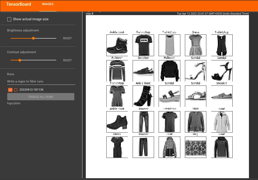

You can also try this code with Online Python Compiler

Run Code

Building Model

model = keras.models.Sequential([
   keras.layers.Flatten(input_shape=(28, 28)),
   keras.layers.Dense(512, activation='relu'),
   keras.layers.Dense(256, activation='relu'),
   keras.layers.Dense(128, activation='relu'),
   keras.layers.Dense(64, activation='relu'),
   keras.layers.Dense(32, activation='relu'),
   keras.layers.Dense(10, activation='softmax')
])

You can also try this code with Online Python Compiler

Run Code

model.compile(loss='sparse_categorical_crossentropy', optimizer='adam', metrics=['accuracy'])

You can also try this code with Online Python Compiler

Run Code

Building a neural network that has five hidden layers. Where each layer has 512, 256, 128, 64, and 32 hidden neurons respectively. To compile the model we will use adam optimizer.

Confusion Matrix Plot

Creating a function that calculates the confusion matrix. To achieve this, you'll utilize a handy Scikit-learn tool and then plot it with matplotlib.

def plot_confusion_matrix(cm, class_names):
 figure = plt.figure(figsize=(8, 8))
 plt.imshow(cm, interpolation='nearest', cmap=plt.cm.Blues)
 plt.title("Confusion Matrix of the Results")
 plt.colorbar()
 tick_marks = np.arange(len(class_names))
 plt.xticks(tick_marks, class_names, rotation=90)
 plt.yticks(tick_marks, class_names)

 labels = np.around(cm.astype('float') / cm.sum(axis=1)[:, np.newaxis], decimals=2)

 threshold = cm.max() / 2.
 for i, j in itertools.product(range(cm.shape[0]), range(cm.shape[1])):
   color = "white" if cm[i, j] > threshold else "black"
   plt.text(j, i, labels[i, j], horizontalalignment="center", color=color)

 plt.tight_layout()
 plt.ylabel('Real Class')
 plt.xlabel('Predicted Class')
 return figure

You can also try this code with Online Python Compiler

Run Code

# Clearing out prior logging data.
!rm -rf logs/image

logdir = "logs/image/" + datetime.now().strftime("%Y%m%d-%H%M%S")
# Defining the basic TensorBoard callback.
tensorboard_callback = keras.callbacks.TensorBoard(log_dir=logdir)
file_writer_cm = tf.summary.create_file_writer(logdir + '/cm')


def log_confusion_matrix(epoch, logs):
 # Using the model to predict the values from the validation dataset.
 test_pred_raw = model.predict(test_images)
 test_pred = np.argmax(test_pred_raw, axis=1)

 # Calculating the confusion matrix.
 cm = sklearn.metrics.confusion_matrix(test_labels, test_pred)
  figure = plot_confusion_matrix(cm, class_names=class_names)
 cm_image = plot_to_image(figure)

 with file_writer_cm.as_default():
   tf.summary.image("Confusion Matrix", cm_image, step=epoch)

# Defining the per-epoch callback.
cm_callback = keras.callbacks.LambdaCallback(on_epoch_end=log_confusion_matrix)

You can also try this code with Online Python Compiler

Run Code

Training the Model

# Starting TensorBoard.
%tensorboard --logdir logs/image

You can also try this code with Online Python Compiler

Run Code

# Training the classifier.
model.fit(
   train_images,
   train_labels,
   epochs=10,
   verbose=0,
   callbacks=[tensorboard_callback, cm_callback],
   validation_data=(test_images, test_labels),
)

You can also try this code with Online Python Compiler

Run Code

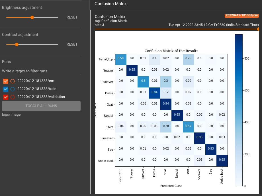
In the above confusion matrix, the x-axis denotes the predicted class, and the y-axis denotes the actual class. We can see that the diagonal elements have a dark blue color; this indicates that the classifier is well trained.

Also, there are some errors in our model, i.e., some T-shirts/tops are classified as Shirts, and some Shirts and Pullovers are classified as Coat.