Do you think IIT Guwahati certified course can help you in your career?
Introduction
This article will discuss the problem of counting the number of non-decreasing arrays C[] with some given constraints.
So, without further ado, let’s jump into the problem statement.
Problem statement
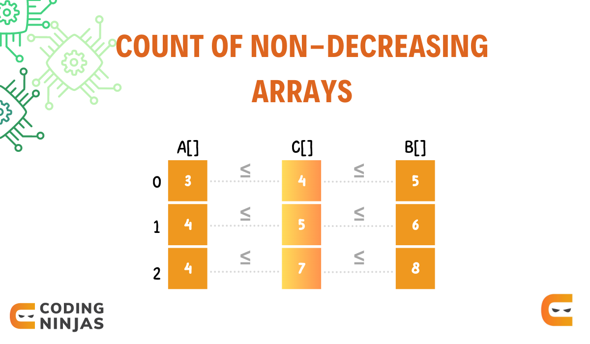
Given two non-decreasing arrays, A[] and B[], of size n, the task is to count the number of non-decreasing arrays C[] of length n, such that the condition A[i] <= C[i] <= B[i], holds for every i in the range [0, n).
In other words, we need to find all possible arrays C[] that are non-decreasing and satisfy the constraint of being within the given lower and upper bounds. An array C is non-decreasing if C[i] <= C[i+1] for every i in the range [0, n-1).
Example
Input
A[] = {3, 4}
B[] = {5, 6}
Output
8
Explanation
All possible arrays that satisfy the condition A[i] <= C[i] <= B[i] are {3, 4}, {3, 5}, {3, 6}, {4, 4}, {4, 5}, {4, 6}, {5, 4}, {5, 5}, {5, 6}.
Out of these nine arrays, all arrays except {5, 4} are non-decreasing. Thus there are eight valid arrays.
Approach 1: Using Recursion
We know that each element of a valid array C[] must be greater than or equal to its previous element.
Let us think of a recurrence relation f(i, j) to solve the given problem recursively.
Let f(i, j) be the number of non-decreasing arrays of length i with their last element in the range [1, j]. The answer to the given problem is f(n, mx) where n is the length of array A[] and B[] and mx is the maximum element in A[] and B[]. Here, f(n, mx) represents the number of non-decreasing arrays of length n, where the last element can have any value in the range [1, mx].
Let’s see the algorithm step-by-step:
Algorithm
We will calculate the maximum element mx from A[] and B[] and use it in the recursive call to find the number of non-decreasing arrays of length n, where the last element is in the range [1, mx].
We will reach the base case of recursion when the length of the required C[] array is 0 (i = 0) because only one array, i.e., the empty array, is valid. More formally, f(i, j) = 1.
No valid array exists if the last element is smaller than the given lower bound. More formally, if i > 0 and j < A[i-1], then f(i, j) = 0.
Now, if the last element is in the given valid range, i.e., greater than A[i-1] and less than B[i-1], then the number of valid arrays can be calculated as the sum of following cases:
The last element equals j. When we fix the last element to j, the element before it has to be less than equal to j. These valid non-decreasing arrays of length i-1, whose last element is less than or equal to j, are given by f(i-1, j).
The last element is smaller than j, i.e., the last element is in the range [1, j-1]. By definition of the recurrence relation, These valid non-decreasing arrays of length i, whose last element is less than or equal to j-1, are given by f(i, j-1).
If the last element is larger than its upper limit, The valid arrays still comprise the arrays with the last element smaller than j. Formally, if i > 0 and j > B[i-1], then f(i, j) = f(i, j-1).
Recurrence relation
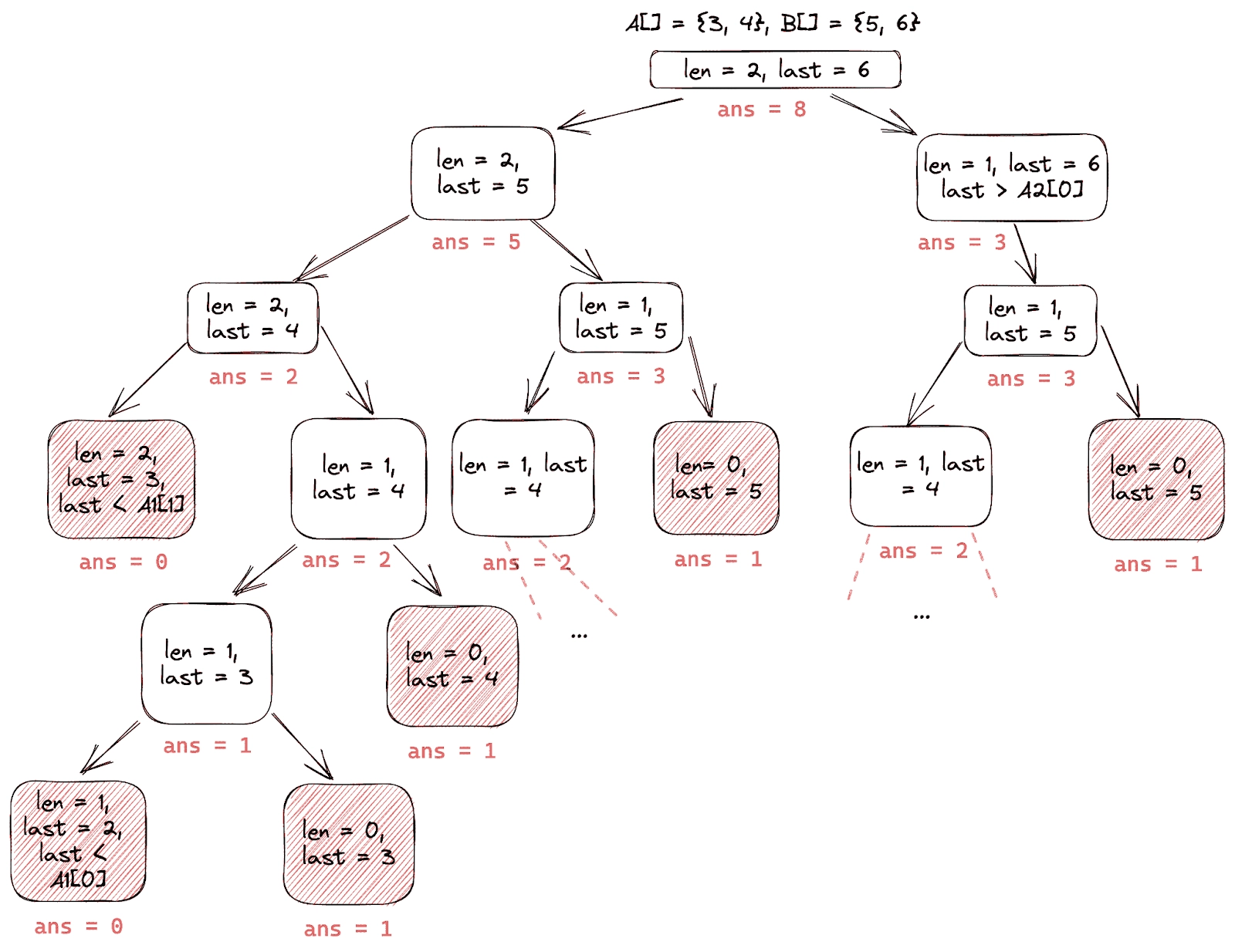
Dry Run
Let’s dry-run the algorithm for the arrays A[] = {3, 4}, B[] = {5, 6} and observe the recursion tree.
Code
#include <bits/stdc++.h>
using namespace std;

int countArraysHelper(vector<int> &A, vector<int> &B, int length, int last) {
   if (length == 0) {
       // Base case: If the length is zero, only one array, which is an empty array
       return 1;
   } else if (last < A[length - 1]) {
       // The last element smaller than lower bound = no array exists
       return 0;
   } else if (A[length - 1] <= last && last <= B[length - 1]) {
       /*
           The last element is within the valid range:
               1. Fix j as the last element
               2. The last element can be in the range [1, j-1]
       */
       return countArraysHelper(A, B, length, last - 1) + countArraysHelper(A, B, length - 1, last);
   } else {
       // Even if j is invalid still contains arrays with smaller last element
       return countArraysHelper(A, B, length, last - 1);
   }
}

// Function to count valid non-decreasing arrays
int countArrays(vector<int> &A, vector<int> &B) {
   int n = int(A.size());

   // Finding maximum element in arrays A[] and B[]
   int mx = 0;
   for (int i = 0; i < n; ++i) {
       if (A[i] > mx)
           mx = A[i];
       if (B[i] > mx)
           mx = B[i];
   }

   // Answer is the number of valid arrays of length n, with the last element in the range [1, mx]
   return countArraysHelper(A, B, n, mx);
}

int main() {
   vector<int> A = {3, 4}, B = {5, 6};
   // vector<int> A = {3, 3, 3}, B = {6, 6, 6};

   // Calling the function
   cout << countArrays(A, B) << '\n';
}
You can also try this code with Online C++ Compiler
In the worst case, the algorithm’s time complexity is O(2^n), where n is the size of the given arrays. At each index of the C[] array, there can be at most two choices, i.e., the last element is j or less than j, which gives the exponential time complexity.
Space Complexity
The algorithm’s space complexity is O(n*mx), where n is the length of input arrays A[] and B[], and mx is the maximum element among all elements in both arrays. Each recursive call takes memory (by creating its stack frame), and there can be n*mx distinct recursive calls.
Approach 2: Using Memoization (Top-Down Approach)
In the previous approach, We can see that we are making recursive calls for overlapping subproblems which cost us more time and increase the time complexity. To reduce the time complexity, We store the result of each recursive call in an array. Before making a new recursive call, we will check if the answer to that recursive call is already present in the array. This technique is called memoization, and now, each unique recursive call is done only once.
Thus, The only difference between this and the previous approach is that, here, a 2D array mem[][] is used to store the results of already done recursive calls. The first dimension (a row) of this 2D array signifies the length of the C[] array, and the second dimension (a column) signifies the largest value of the last element of the C[] array.
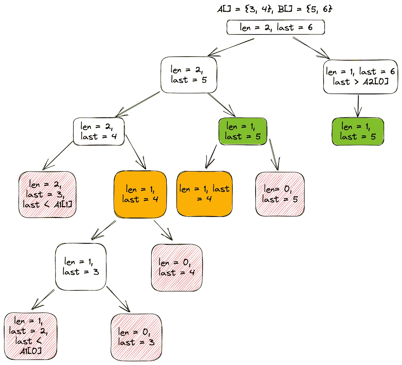
Dry Run
Let’s dry-run the algorithm for the arrays A[] = {3, 4}, B[] = {5, 6} and observe the recursion tree with recursive calls for overlapping subproblems.
Orange and green colour boxes represent the recursive calls for overlapping subproblems.
Code
#include <bits/stdc++.h>
using namespace std;

int countArraysHelper(vector<int> &A, vector<int> &B, int length, int last, vector<vector<int>> &mem) {
   if (length == 0) {
       // Base case: If the length is zero, only one array, which is an empty array
       return 1;
   }

   // If the result of that recursive call is already present
   if (mem[length][last] != -1) {
       return mem[length][last];
   }

   int ans;
   if (last < A[length - 1]) {
       // last element smaller than lower bound = no array exists
       ans = 0;
   } else if (A[length - 1] <= last && last <= B[length - 1]) {
       /*
           The last element is within the valid range:
               1. Fix j as the last element
               2. The last element can be in the range [1, j-1]
       */
       ans = countArraysHelper(A, B, length, last - 1, mem) + countArraysHelper(A, B, length - 1, last, mem);
   } else {
       // Even if j is invalid still contains arrays with smaller last element
       ans = countArraysHelper(A, B, length, last - 1, mem);
   }

   // Store the answer for a recursive call in the 2D array
   mem[length][last] = ans;
   return ans;
}

// Function to count valid non-decreasing arrays
int countArrays(vector<int> &A, vector<int> &B) {
   int n = int(A.size());

   // Finding the maximum element in arrays A[] and B[]
   int mx = 0;
   for (int i = 0; i < n; ++i) {
       if (A[i] > mx)
           mx = A[i];
       if (B[i] > mx)
           mx = B[i];
   }

   // Forming the table for storing the results of recursive calls
   vector<vector<int>> mem(n + 1, vector<int>(mx + 1, -1));

   // Answer is the number of arrays of length n, with the last element in the range [1, mx]
   return countArraysHelper(A, B, n, mx, mem);
}

int main() {
   vector<int> A = {3, 4}, B = {5, 6};
   // vector<int> A = {3, 3, 3}, B = {6, 6, 6};

   // Calling the function
   cout << countArrays(A, B) << '\n';
}
You can also try this code with Online C++ Compiler
The algorithm’s time complexity is O(n*mx), where n is the length of input arrays A[] and B[], and mx is the maximum element among all elements in both arrays because we do each recursive call only once, and there are n*mx unique recursive calls.
Space Complexity
The algorithm’s space complexity is O(n*mx), where n is the length of input arrays A[] and B[], and mx is the maximum element among all elements in both arrays because the 2D array consumes space, used to store the result of recursive calls.
Approach 3: Using DP (Bottom-Up Approach)
To solve this problem using Dynamic Programming, we have to take a 2D array where:
Rows signify the length of the required C[] array.
Columns signify the range of the last element of the C[] array.
In this approach, dp[i][j] = the number of non-decreasing arrays C[] satisfying given constraints such that the last element is in the range [1, j].
Let’s see the algorithm step-by-step:
Algorithm
Find the maximum element mx among all elements in arrays A[] and B[].
Make a 2D array dp[][] having n+1 rows and mx+1 columns (1-based indexing).
Initialise the number of arrays with zero length and any last element to 1. As only one array - the empty array has zero length. Initialise all remaining elements of the array to 0.
According to the recurrence relation, dp[i][j] depends on dp[i][j-1] and dp[i-1][j]. Now, we traverse the dp[][] array in such a way that dp[i][j-1] and dp[i-1][j] are calculated before dp[i][j].
Find the value of dp[i][j] using the recurrence relation according to the satisfied condition.
Code
#include <bits/stdc++.h>
using namespace std;

// Function to count number of valid non-decreasing arrays
int countArrays(vector<int> &A, vector<int> &B) {
   int n = int(A.size());

   // Finding the maximum element in arrays A[] and B[]
   int mx = 0;
   for (int i = 0; i < n; ++i) {
       if (A[i] > mx)
           mx = A[i];
       if (B[i] > mx)
           mx = B[i];
   }

   // 2D array for storing the results
   vector<vector<int>> dp(n + 1, vector<int>(mx + 1, 0));

   for (int i = 0; i <= mx; ++i) {
       // Base case: If the length is zero, we get only one array, i.e. the empty array
       dp[0][i] = 1;
   }

   // Traversing the 2D dp array
   for (int i = 1; i <= n; ++i) {
       for (int j = 1; j <= mx; ++j) {
           if (j < A[i - 1]) {
               // The last element smaller than lower bound = no array exists
               dp[i][j] = 0;
           } else if (A[i - 1] <= j && j <= B[i - 1]) {
               /*
                   The last element is within the valid range:
                       1. Fix j as the last element
                       2. The last element can be in the range [1, j-1]
               */
               dp[i][j] = dp[i][j - 1] + dp[i - 1][j];
           } else {
               // Even if j is invalid still contains arrays with smaller last element
               dp[i][j] = dp[i][j - 1];
           }
       }
   }

   // Answer is the number of arrays of length n, with the last element in the range [1, mx]
   return dp[n][mx];
}

int main() {
   vector<int> A = {3, 4}, B = {5, 6};
   // vector<int> A = {3, 3, 3}, B = {6, 6, 6};

   // Calling the function
   cout << countArrays(A, B) << '\n';
}
You can also try this code with Online C++ Compiler
The algorithm’s time complexity is O(n*mx), where n is the length of input arrays A[] and B[], and mx is the maximum element among all elements in both arrays because we traverse a 2D array of size n*mx only once.
Space Complexity
The algorithm’s space complexity is O(n*mx), where n is the length of input arrays A[] and B[], and mx is the maximum element among all elements in both arrays because we use a 2D array of size n*mx.
Approach 4: Using Space-Optimised DP
In the previous DP approach, we can observe that the answer is only dependent on the current and previous dp array (dp[i][j] depends on the value of dp[i][j-1] and dp[i-1][j]). Thus we can solve the problem using two one-dimensional dp arrays and optimise the space complexity.
Let’s see the algorithm step-by-step:
Algorithm
Initialise a dp array prev of mx+1 size with 1 (The base case). Currently, this prev array represents the array dp[0].
Create another dp array curr, which stores the dp array for the next level after prev.
The curr array is calculated in the same way using the recurrence relation. All occurrences of dp[i-1][j] can be replaced by prev[j], and all occurrences of dp[i][j-1] can be replaced by curr[j-1].
After computing the current row curr, the array is assigned to prev. And similarly, a new curr array is calculated for the next row.
This way, the dp array for all rows is computed level by level.
Code
#include <bits/stdc++.h>
using namespace std;

// Function to count number of valid non-decreasing arrays
int countArrays(vector<int> &A, vector<int> &B) {
   int n = int(A.size());

   // Finding the maximum element in arrays A[] and B[]
   int mx = 0;
   for (int i = 0; i < n; ++i) {
       if (A[i] > mx)
           mx = A[i];
       if (B[i] > mx)
           mx = B[i];
   }

   // 1D arrays for storing the results
   vector<int> prev(mx + 1), curr(mx + 1);
   for (int i = 0; i <= mx; ++i) {
       // Base case: If the length is zero, we get only one array, i.e. the empty array
       prev[i] = 1;
   }

   for (int i = 1; i <= n; ++i) {
       for (int j = 1; j <= mx; ++j) {
           if (j < A[i - 1]) {
               // The last element smaller than lower bound = no array exists
               curr[j] = 0;
           } else if (A[i - 1] <= j && j <= B[i - 1]) {
               /*
                   The last element is within the valid range:
                       1. Fix j as the last element
                       2. The last element can be in the range [1, j-1]
               */
               curr[j] = curr[j - 1] + prev[j];
           } else {
               // Even if j is invalid still contains arrays with smaller last element
               curr[j] = curr[j - 1];
           }
       }
       prev = curr;
   }

   // Answer is the number of ways to get an array of length n, with the last element in the range [1, mx]
   return curr[mx];
}

int main() {
   vector<int> A = {3, 4}, B = {5, 6};
   // vector<int> A = {3, 3, 3}, B = {6, 6, 6};

   // Calling the function
   cout << countArrays(A, B) << '\n';
}
You can also try this code with Online C++ Compiler
The algorithm’s time complexity is O(n*mx), where n is the length of input arrays A[] and B[], and mx is the maximum element among all elements in both arrays because of the for loops.
Space Complexity
The algorithm’s space complexity is O(mx), where mx is the maximum element among all elements in both arrays because we use two one-dimensional arrays of length mx.
Frequently Asked Questions
What is a non-decreasing array?
An array A is non-decreasing if A[i] <= A[i+1] for every i in the range [0, n-1).
What is dynamic programming?
Dynamic programming is a technique where the problem is broken into sub-problems so that their results can be reused to obtain the optimal solution.
What is memoization?
To reduce the time complexity, We store the result of each recursive call in an array. Before making a new recursive call, we will check if the answer to that recursive call is already present in the array. This technique is called memoization, and now, each unique recursive call is done only once.
Why should I use memoization when I have solved this question using recursion?
When you use recursion, you might repeat the exact computations repeatedly (as we saw above), which leads to exponential time complexity. Memoization reduces the number of function calls required, making code more efficient.
How is the Bottom-Up approach better than the Top-Down approach?
The Bottom-Up approach is considered better than the Top-Down approach as there is no recursion overhead in the Bottom-Up approach, unlike the Top-Down approach. The Top-Down approach also runs the risk of stack overflow if the number of recursive calls is too high, unlike the Bottom-Up approach.
Conclusion
In this article, we solved the problem statement to Count permutations of the given array that generates the same Binary Search Tree (BST). Along with the solution, we also discussed the time and space complexity of the solution.
If you want to learn more about Binary search trees and want to practice some questions which require you to take your basic knowledge on these topics a notch higher, then you can visit our Guided Path for arrays on Coding Ninjas Studio. To be more confident in data structures and algorithms, try out our DS and Algo Courses. Until then, All the best for your future endeavours, and Keep Coding.


 9+ registered

