Data Flow Analysis in Compiler Design

Introduction

In compiler design, code optimization is a program transformation technique that tries to improve the intermediate code to consume fewer resources such as CPU, memory, etc., resulting in faster machine code.

There are two types of code optimization techniques.

1. Local optimization- This code optimization applies to a small block of statements. Examples of local optimization are variable/constant propagation and common subexpression elimination.
2. Global optimization- This code optimization applies to large program segments like functions, loops, procedures etc. An example of global optimization is data flow analysis.

This article will discuss a global optimization technique, i.e. data flow analysis.

Data Flow Analysis

Data flow analysis is a global code optimization technique. The compiler performs code optimization efficiently by collecting all the information about a program and distributing it to each block of its control flow graph (CFG). This process is known as data flow analysis.

Since optimization has to be done on the entire program, the whole program is examined, and the compiler collects information.

Note: The control flow graph represents a program in blocks depicting how the control of the program is being passed from one block to another.

We will proceed with our discussion with some basic terminologies in data flow analysis.

Basic Technologies

Below are some basic terminologies related to data flow analysis.

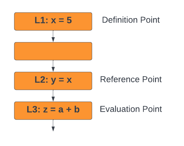
• Definition Point- A definition point is a point in a program that defines a data item.
• Reference Point- A reference point is a point in a program that contains a reference to a data item.
• Evaluation Point- An evaluation point is a point in a program that contains an expression to be evaluated.

The below diagram shows an example of a definition point, a reference point, and an evaluation point in a program.

Next, we will discuss the data flow analysis equation.

Also See, Top Down Parsing

Data Flow Analysis Equation

The data flow analysis equation is used to collect information about a program block. The following is the data flow analysis equation for a statement s-

Out[s] = gen[s] U In[s] - Kill[s]

where

Out[s] is the information at the end of the statement s.

gen[s] is the information generated by the statement s.

In[s] is the information at the beginning of the statement s.

Kill[s] is the information killed or removed by the statement s.

The main aim of the data flow analysis is to find a set of constraints on the In[s]’s and Out[s]’s for the statement s. The constraints include two types of constraints- The transfer function and the Control Flow constraint.

Let’s discuss them.

Transfer Function

The semantics of the statement are the constraints for the data flow values before and after a statement.

For example, consider two statements x = y and z = x. Both these statements are executed.

Thus, after execution, we can say that both x and z have the same value, i.e. y.

Thus, a transfer function depicts the relationship between the data flow values before and after a statement.

There are two types of transfer functions-

1. Forward propagation
2. Backward propagation

Let’s see both of these.

• Forward propagation
  • In forward propagation, the transfer function is represented by Fs for any statement s.
  • This transfer function accepts the data flow values before the statement and outputs the new data flow value after the statement.
  • Thus the new data flow or the output after the statement will be Out[s] = Fs(In[s]).
• Backward propagation
  • The backward propagation is the converse of the forward propagation.
  • After the statement, a data flow value is converted to a new data flow value before the statement using this transfer function.
  • Thus the new data flow or the output will be In[s] = Fs(Out[s]).

Control-Flow Constraints

The second set of constraints comes from the control flow. The control flow value of Si will be equal to the control flow values into Si + 1 if block B contains statements S1, S2,........, Sn. That is:

IN[Si + 1] = OUT[Si], for all i = 1 , 2, .....,n – 1.

Now, we will discuss some data flow properties.

Data Flow Properties

Some properties of the data flow analysis are-

• Available expression
• Reaching definition
• Line variable
• Busy expression

We will discuss these properties one by one.

Available Expression

An expression a + b is said to be available at a program point x if none of its operands gets modified before their use. It is used to eliminate common subexpressions.

An expression is available at its evaluation point.

Example: 

In the above example, the expression L1: 4 * i is an available expression since this expression is available for blocks B2 and B3, and no operand is getting modified.

Reaching Definition

A definition D is reaching a point x if D is not killed or redefined before that point. It is generally used in variable/constant propagation.

Example:

In the above example, D1 is a reaching definition for block B2 since the value of x is not changed (it is two only) but D1 is not a reaching definition for block B3 because the value of x is changed to x + 2. This means D1 is killed or redefined by D2.

Live Variable

A variable x is said to be live at a point p if the variable's value is not killed or redefined by some block. If the variable is killed or redefined, it is said to be dead.

It is generally used in register allocation and dead code elimination.

Example:

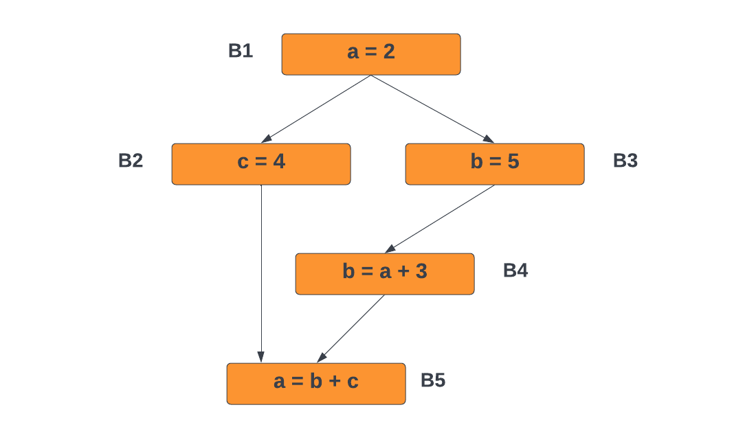
In the above example, the variable a is live at blocks B1,B2, B3 and B4 but is killed at block B5 since its value is changed from 2 to b + c. Similarly, variable b is live at block B3 but is killed at block B4.

Busy Expression

An expression is said to be busy along a path if its evaluation occurs along that path, but none of its operand definitions appears before it.

It is used for performing code movement optimization.