Data Preprocessing - Introduction

Data Cleaning

Data cleaning is the process of handling the missing values or incorrect values that may be distractive for our model. 

Handling missing values

The dataset can contain missing values. This may be handled manually, however might not be feasible when the dataset is huge (which it generally is in a real-world scenario). Missing values may be denoted by ‘NaN’ or ‘NA’ in the dataset. These empty values can be filled with the mean or the median of that feature. Generally, in normally distributed data we use mean, while in non-normal distribution median is preferred.

So suppose we have a missing value in feature, number of rooms in a house. It’s an ideal case where we may use the mean of all the values in the feature column to fill the empty values. 

Handling Noise

Noisy data is the one that contains random errors or unnecessary data points. Mentioned below are some of the techniques to handle the problem of noise:-

Binning 

It is used to minimise the effects of observation error. Binning converts continuous values to their corresponding categorical counterpart. Let us understand through an example.

Say, We have a feature called Age with following values {19, 5 , 10 , 33, 63 ,72 ,18 , 42 , 26, 82, 11, 17}

We’ll create a bin of fix width say 10. 

bins= { 0 {0-9}, 1 {10-19}, 2 {20-29}, 3 {30-39}, …..}

So after binning our Age feature would look like 

{ 1, 0, 1, 3, 6, 7, 1, 4, 2, 8, 1, 1}

This technique also helps in easily identifying and segregating outliers. 

Clustering

The process involves forming groups of similar values in a dataset. The values that don’t fit into any group are considered noise and are removed. We may use K-means to form the clusters.

Dealing with Outliers

Outliers are values which show an extremely unusual variation(which may be a result of human error) from the general trend and hence can make the model very skewed. These values are rare but can make a significant impact on our model and can therefore be safely scrapped off. There are various techniques that may be used to deal with the problem of outliers. 

Z-score 

Z-score = (data point - mean) /  standard deviation

Z score checks for values showing significant skewness. We set a threshold value over which the z score classifies a datapoint as an outlier. 

Data visualisation 

It is another widely used method to check for outliers. Various graphical methods may be used -

1. Histograms
2. Scatter plot
3. Box plot

Data Transformation

This is the next step in the preprocessing phase.  Data transformation is the stage where the dataset is made suitable to be used for training. This may involve using alternate values or changing the format. This step is essential since machine learning models need to be fed data in a specific format to work efficiently. 

There are various techniques for data transformation:-

Normalisation

Normalisation is a technique of scaling data to fit within a range so as to make it suitable for model training. Normalisation transforms numeric values to fit a fixed range without loss of information. Consider a feature that contains values ranging from 100 to 10000. We may want to normalise the data and fit all the values to a corresponding value in range of [0,1]. This not only scales down the huge difference between the datapoints which could’ve distorted the model during training but also retains essential information about the datapoints. There are various techniques to normalise the data - 

Min-max normalisation 

It is given by the formula 

Z = (x - min(x)) / max(x) - min(x)

This scales down the values to a [0,1] range where the maximum value in the dataset is equivalent 1 while the minimum value is equivalent to 0. 

Z-score normalisation 

The values are transformed using the formula-

Z = (X - mean(x)) / stdev(x)

Data Encoding

It is an integral step in the data transformation stage. Often features have values which are not suitable to be processed by the model. It is used to transform categorical features into a corresponding numeric value. For example, the dataset may have gender features with values either as ‘male’ or ‘female’. These string values can’t be efficiently processed by the model so they need to be converted to some numeric value. This process is known as data encoding. There are various data encoding techniques- 

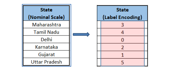
Label encoding 

Label encoding maps every categorical value in a given feature to a unique numeric value. 

Source- link

One-hot Encoding 

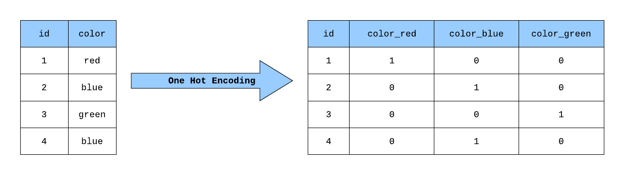
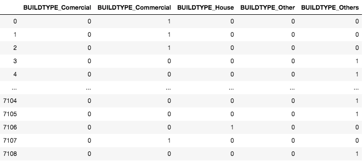
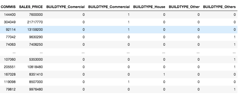
It is another widely used data encoding technique that makes use of dummy columns to represent the value in the categorical feature. Every categorical variable makes up a dummy variable or dummy column. The values in dummy features are taken as 1 if they are in the original dataset, otherwise 0. See the example below.

Source- link

Data Reduction

Although machine learning algorithms are data-driven and it’s a common perception that more the data, better the accuracy. However, often times the dataset might be unnecessarily huge. This redundancy in data doesn’t necessarily improve the accuracy significantly but it makes processing more cumbersome. In that case, it makes sense to get rid of redundant data. There are various techniques to handle the problem of data redundancy. 

Dimensionality reduction 

Dimensionality refers to the features of a given dataset. An unnecessarily huge data may lead to a problem of dimensionality known as ‘Curse of dimensionality’. More the dimensionality, theoretically implies more data which as per common perception would lead to better results. However, A higher order dimensionality may not be feasible to comprehend even on a machine. The tools at present are designed to anaylse 2D or 3D relations. Anything beyond that is counter intuitive and hence it makes computation far more complex without practically deriving anything significant from the dataset.  Dimensionality Reduction aims to perform feature extraction. This technique reduces redundant features or attributes in a dataset that might not make a significant impact on the final predictions. This can be done by principal component analysis. PCA defines a new set of variables from the existing variable which are called principal components. It is a linear combination of original features and the components are extracted in a way such that the first PC captures the maximum variance in the dataset, followed by second and so on. Independent variables showing some correlation are likely to be discarded. 

Discretisation 

This involves grouping similar values in the dataset to be represented by a group it is associated with. For example, a dataset has an Age feature with values ranging from 5 to 100. We may want to group the individuals as children, adults, and senior citizens based on their age. For children an age range of 5 - 18, for adults 18 - 60, for senior citizens >60. Discretisation works on a similar basis as binning. 

 

Data Reduction is the final step in the data preprocessing phase. 

Sometimes, our training data may be heavily dominated by the majority class. This may lead to our model totally ignoring the minority class. This is known as the Imbalanced Classification problem. This is a major problem since the minority class might be of utmost importance. Let’s say we have data to check for people who failed to repay the loan. Now it’s safe to assume that there would be more regular loan payees than defaulters if the bank is doing well. In this case, the defaulters would make up our minority class and they would be more of our interest than regular payees. Remember, in this case, we can afford to have more false positives than false negatives. That is, the bank would rather prefer not to sanction a loan to a person who’s not likely to falter rather than extend a loan to someone who might. 

To deal with this problem, there 2 common techniques:-

1. Oversampling:- making copies of minority class samples. Oversampling is one method but it has its disadvantages. Since it makes copies of already existing data points, it’s never a good idea to feed the same sample to the model again. This may lead to overfitting. However, it can be given a shot. 
2. Undersampling:- A more sensible approach where we remove samples from the majority class. This may somewhat balance out the ratio without having to worry about the problem of overfitting.

Implementation 

We have learnt and understood all stages in the preprocessing phase we need to go through. Now let’s jump into python implementation. You can find the dataset here.

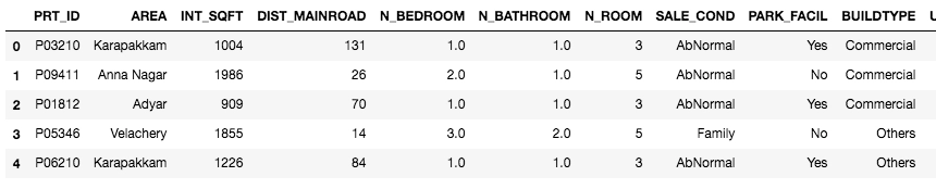
To begin with the preprocessing stage, we first need to explore the initial data. 

import pandas as pd
import numpy as np
import matplotlib.pyplot as plt
%matplotlib inline

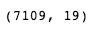
df = pd.read_csv("chennai_house_price_prediction.csv")
df.shape

 

df.head()

 

df.describe(include='all')

 

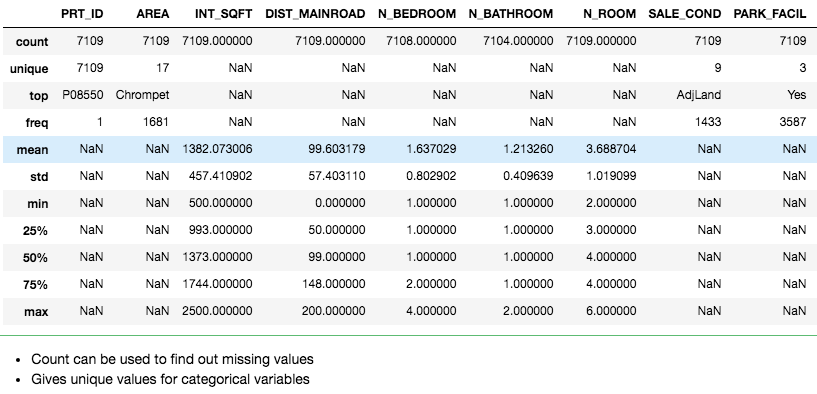
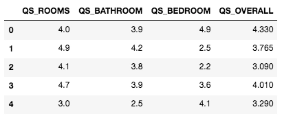
describe function provides basic statistical data about the dataset like mean, count, percentiles, etc and is an excellent method to explore the initial data. 

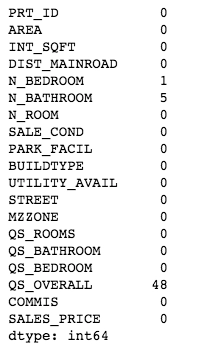
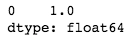
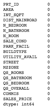
df.isnull().sum()

 

Isnull function detects missing values. Sum function sums up the total number of missing values in the feature. 

temp = pd.DataFrame(index=df.columns)
temp['data_type'] = df.dtypes
temp['null_count'] = df.isnull().sum()
temp['unique_count'] = df.nunique()
print(temp)

 

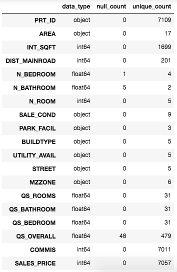
 We created a temp dataframe to visualise data_type, total null values and total unique values for every feature in the dataset. Now we know how many features we have with missing values.

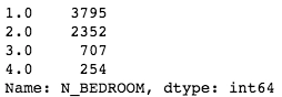
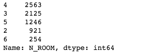
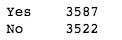
Value_counts function gives out frequency of unique value in a feature.

df['N_BEDROOM'].value_counts()

 

• It has four different categories
• This variable should be object and not integer
   

df['N_BEDROOM'].value_counts()/len(df)*100

 

• About 53% houses have one bedroom
• 33% have 2 bedrooms
• Less than 10% houses have 3 bedrooms
• Only 3.5% have 4 bedrooms
   

df['N_ROOM'].value_counts()

 

The 'Rooms' might have a number of kitchen, hall, dining area etc.

No house with 1 room, and a very few that have 2

df['N_BATHROOM'].value_counts()/len(df)

 

78% houses have 1 bathroom and 21% have 2 bathrooms

df['PARK_FACIL'].value_counts()

 

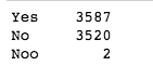
We can see that the number of houses with and without parking facility is similar. And we can see 2 values with ‘Noo’ instead of ‘No’. We will treat that later. 

Now we will manipulate data. We will fix the following issues with the dataset. 

1. Drop Duplicates (if any)
2. Fill the missing Values
3. Correct the data types
4. Fix the spelling errors in variables

 

df.drop_duplicates()
df.shape()

 

We had no duplicates. Hence the shape did not change.

Now we will deal with missing values. 

df.isnull().sum()

 

Different ways deal with the missing values

• Remove the rows with missing values
• Mean or median in case of continuous variable
• With mode in case of categorical variable
• Using other independent variables
   

We’ll refrain from dropping data as much as possible if other methods can be conveniently employed. 

df['N_BEDROOM'].mode()

 

For missing values in N_BEDROOM, we’ll use the mode value of the feature. Which is 1 in this case. 

df['N_BEDROOM'].fillna(value = (df['N_BEDROOM'].mode()[0]), inplace=True)

 

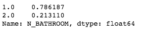
We have 5 missing values in N_BATHROOM which we’ll fill based on the number of bedrooms in that house. 

for i in range(0, len(df)):
    if pd.isnull(df['N_BATHROOM'][i])==True:
        if (df['N_BEDROOM'][i] == 1.0):
            df['N_BATHROOM'][i] = 1.0
        else: 
            df['N_BATHROOM'][i] = 2.0

 

df[[ 'QS_ROOMS','QS_BATHROOM', 'QS_BEDROOM', 'QS_OVERALL']].head()

 

For missing values in QS_OVERALL we’ll take the mean of the other 3 quality scores. 

temp = (df['QS_ROOMS'] + df['QS_BATHROOM'] + df['QS_BEDROOM'])/3
pd.concat([df['QS_ROOMS'], df['QS_BATHROOM'], df['QS_BEDROOM'], temp], axis=1).head(10)

 

We’ll map the corresponding temp value to QS_OVERALL where the datapoint is missing.

def fill_na(x):
    return ((x['QS_ROOMS'] + x['QS_BATHROOM'] + x['QS_BEDROOM'])/3)
df['QS_OVERALL'] =  df.apply(lambda x: fill_na(x) if pd.isnull(x['QS_OVERALL']) else x['QS_OVERALL'], axis=1)
df.isnull().sum()

  

So we have taken care of all the missing values in the dataset. 

df['PARK_FACIL'].replace({'Noo':'No'}, inplace = True) df['PARK_FACIL'].value_counts()

buildtype= pd.get_dummies(df.BUILDTYPE, prefix='BUILDTYPE')
buildtype

 

df = pd.concat([df, buildtype], axis=1)
df

 

We may encode all the string categorical variables. We’ll leave that as an exercise for you. 

Frequently Asked Questions

1. Why do we need to preprocess the data? 
   Ans. In the real world, it’s unlikely to get a training-ready data. Most of the times this data contains missing variables, erroneous data which needs to be treated before it is ready to be used. 
    
2. What is categorical data encoding and why is it essential? 
   Ans. Categorical data encoding is a process of mapping unsuitable data type values to suitable numeric value which can be efficiently processed by our training model. As the name suggests, it is only done for categorical features. 
    
3. Briefly explain the steps in data preprocessing phase. 
   Ans. First we need to explore the data to know what all feature need to treated for missing values, data encoding, outliers etc. Then we manipulate the data accordingly to make it suitable for training. 

Key Learnings

Data preprocessing is unavoidable and one of the essential stages in model building. A well put data can significantly improve accuracy scores of a model. In this blog, we have covered data preprocessing in detail, and we strongly advise you to implement the code yourself to get a better understanding of how to go about it. As a Data scientist, recruiters expect you to have a mastery over data preprocessing. You can check out our expert-curated course on machine learning and data science to ace your next Data science interview.