Do you think IIT Guwahati certified course can help you in your career?
Introduction
Decision Trees: Decision Trees are the Supervised Machine learning algorithm that can be used for Classification and Regression problems. A classification problem identifies the set of categories or groups to which an observation belongs. A Decision Tree uses a tree or graph-like model of decision.
Each internal node represents a "test" on attributes, and each branch represents the outcome of the test. Each leaf node represents a class label (decision taken after computing all features).
Why Decision Tree Structure in ML?
A decision tree is a widely used algorithm in machine learning that represents decisions and their possible outcomes in a tree-like format. It works by splitting data into branches based on specific attribute values. Each internal node tests a feature, each branch represents the outcome of that test, and each leaf node delivers a final output or prediction.
Decision trees are highly interpretable, making it easy to understand the reasoning behind each prediction. They support both classification and regression tasks and can handle numerical as well as categorical data. Thanks to their versatility, clarity, and minimal preprocessing needs, decision trees are often preferred for building fast, explainable, and effective predictive models.
Common Examples
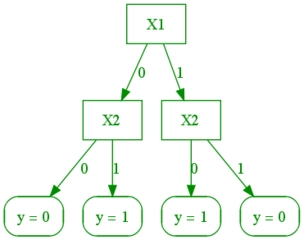
Let's draw a Decision Tree for calculating the XNOR table. The table is as follows:
INPUT-1
X1
INPUT-2
X2
OUTPUT
Y
1
1
1
1
0
0
0
1
0
0
0
1
Here, we have three features: INPUT-1, INPUT-2, and OUTPUT.
Let's make the feature INPUT-1 the root node and build a Decision Tree.
Here we have split our features at each level depending upon the requirement, and at last, we have final decisions. In actual practice, the data is not as simple as this. The complexity of trees would increase as the data tend towards more practical real-world examples. Let's have a look at a similar kind of example:
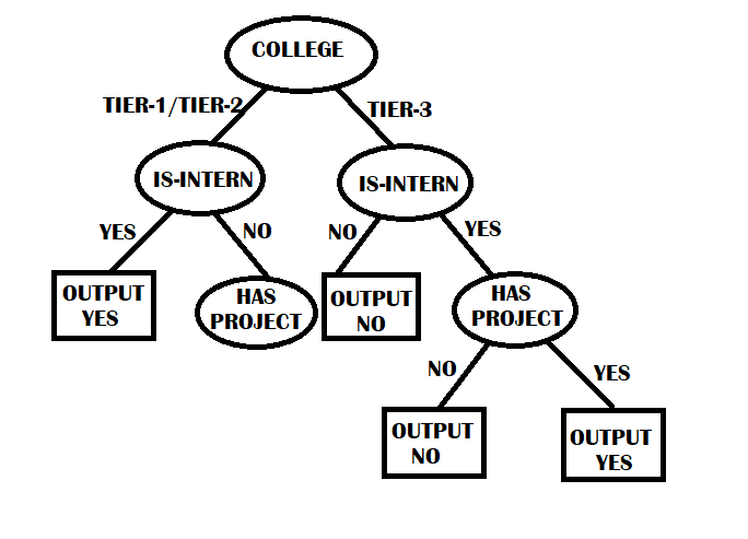
Suppose we have to predict whether a student has been invited for an interview or not. We have three features, college type, is-intern, and has-project, and based on these, we have to make the Decision Tree.
TIER-1/TIER-2
TIER-3
IS-INTERN
HAS-PROJECT
GOT A CALL
YES
YES
YES
YES
YES
YES
NO
YES
YES
NO
YES
YES
YES
NO
NO
NO
YES
YES
NO
NO
YES
NO
YES
NO
YES
YES
YES
YES
In the Machine Learning algorithm, we try to find a nearly accurate result and not the exact one. The task would be very complex if we train the algorithm to get the precise result every time. Similarly, the best version of the Decision Tree is very expensive and computationally impossible to build. So we try to develop a perfect Decision Tree that will give decent accuracy and be much easier to make. According to the above Decision Tree, if a student is from tier-3 college and has a fantastic internship(say Google) but doesn't have any project, they will not get an interview call, which is practically not feasible. Mistakes will come in the way when we have exceptions that don't match the data upon which the Decision Tree is built.
Mathematics behind Decision Tree:
The following are the steps that we need to follow to build a very good Decision Tree:-
1) We need to select the target attribute/feature from the given attributes. In the above example, the target attribute is “GOT A CALL,” which has two classes of values, either yes or no.
2) Calculate the information gain of the selected target attribute
Information Gain = -PP+N log2(PP+N) - NP+N log2(NP+N)
Where P = number of the elements in class 1 of the target attribute.
N = number of the elements in class 2 of the target attribute.
In our case, the target attribute has two classes, “YES” and “NO”. So, P=5, and N=5.
3) Now for the remaining features/attributes.
We calculate the entropy for all the Categorical variables.
We take average information entropy for the current attribute.
The entropy of a given attribute is given by:
Entropy = i=1v Information gain of that i th categorical variable x Probability of i th categorical variable
Here 'V is the number of categorical variables in that attribute.
For example, if the attribute is "IS-INTERN," then it has two categorical variables, "YES" and "NO."
I.G of “YES” = -47log2(47) say E1
I.G of “NO” = -37log2(37) say E2
The entropy of the attribute “IS-INTERN” = E1+E2
4) Wel will now find the Gain of each attribute (except the target attribute).
Gain of Individual attribute = Information Gain of the target attribute - Entropy of that attribute.
5) The attribute having maximum Gain value will be our Root node. We will divide the root node into subsets that contain possible values for the best feature.
6) Recursively make new decision trees using the subsets of the dataset created in step 5, till the point where we don't have any features to split upon.
Implementation
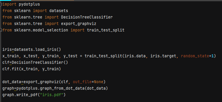
Now we will see the implementation of the Decision Tree using Scikit-Learn.
clf.fit(x_train, y_train)is used to build the Decision Tree. Once the tree is built, we can export this into the pdf. To do this, I import a function from sklearn.tree import exportgraphviz
We supply the classifier clf to the function export_graphviz(clf, out_file=None). out_file=Nonemeans I don't want to save the output into any external file. I want this function to return the data. The function’s output is the dot () data, and then I want to export it into a dot pdf.
pydotplus.graph_from_dot_data(dot_data) returns a pydot object which I have taken in a graph object.
graph.write_pdf() is a method to assign the name of the pdf.
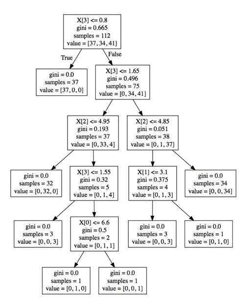
Output
Advantages of Decision Trees
Easy to Interpret and Visualize Decision trees follow a hierarchical structure and use Boolean logic, making them extremely easy to understand and interpret. Even individuals without technical knowledge can follow the decision-making process from root to leaf. This interpretability makes them popular for applications where explainability is essential.
Minimal Data Preparation Required Decision trees can handle both categorical and numerical data and are tolerant of missing values. Unlike many machine learning algorithms, they require little to no normalization or scaling of data, making preprocessing easier and saving development time.
Versatile and Robust Decision trees are suitable for both classification and regression problems. They are also relatively insensitive to the correlation between features, which is beneficial when dealing with datasets that have highly interdependent variables.
Disadvantages of Decision Trees
Prone to Overfitting One of the biggest drawbacks of decision trees is their tendency to overfit, especially with complex datasets. Overfitting occurs when the model becomes too tailored to training data and loses generalization. Pruning techniques, like reduced error pruning or cost-complexity pruning, are used to address this issue by trimming branches that add little predictive power.
High Variance Decision trees are unstable, meaning small changes in the dataset can result in entirely different tree structures. This high variance affects model reliability. Ensemble techniques like Random Forest help overcome this by averaging multiple trees.
Computationally Expensive to Train The training process of a decision tree involves evaluating all possible splits at each node, which is a greedy and resource-intensive approach. As the dataset grows, this makes training slower and more computationally expensive.
Frequently Asked Questions
What are the advantages of a Decision Tree?
Ans. Following are the advantages of Decision Tree
As the implementation is like a binary tree, the time complexity for building and querying is very less.
Very easy to build.
The implementation is non-linear, so the accuracy is high.
It can handle both continuous and discrete data.
What are the disadvantages of a Decision Tree?
Ans. a) Memory consumption is very high as the calculation requires lots of variables b) Very expansive to create c) Less appropriate for predicting the continuous values d) It often lead to overfitting of the data, which can give the wrong prediction on the testing data
What are the different types of nodes in the Decision Tree?
Ans. a) Root node: It is the uppermost node in the Decision Tree. b) Decision nodes: Decision node helps in split the data into multiple segments c) Leaf nodes: The final output is obtained from the leaf nodes.
How does a Decision Tree handle the missing values of an attribute?
Ans. a) It fills the missing values by the most common value of that attribute b) It fills the missing values by assigning a probability to each of the attribute's possible values based on the other samples.
What are the standard algorithms used for deriving the Decision Tree?
Ans. The standard algorithms are:
ID3(Iterative Dichotomiser)
C4.5 (Successor of ID3)
CART ( Classification and Regression Trees)
Conclusion
I hope this article helped you clearly understand the concept and implementation of Decision Tree algorithms. While Decision Trees are a powerful tool in Machine Learning, there are many other exciting algorithms worth exploring. If you're interested, consider diving deeper into other popular ML techniques to expand your knowledge further


 9+ registered

