Deep Convolutional Generative Adversarial Networks

Strided Convolution

Source

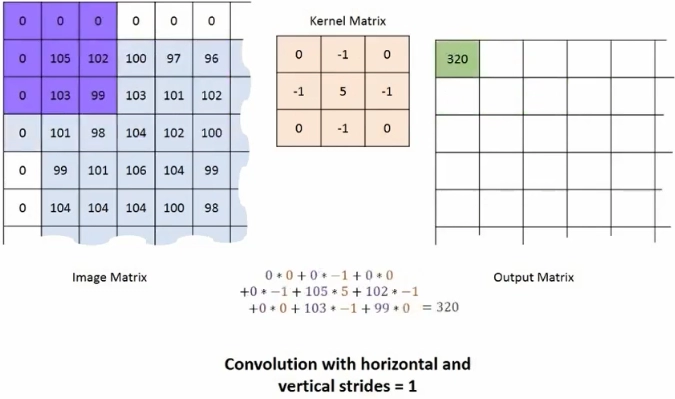
If you slide the window one pixel at a time, this is called a convolution of stride equals 1. On the other hand, if the window is sled two pixels along with the horizontal and vertical directions,  this is called convolution with stride equals two or more commonly stridden convolutions. It turns out that these techniques allow GANs to learn better down and upsampling filters.

In basic GANs,  we have used sigmoid activations at the output layer to squash the values between zeros and ones. In deep convolutional GANs, I recommend using Tan(h) activation. It will result in values squashed between negative and positive ones. It was found empirically that this produced more appealing results. However, we should not forget to scale the importance of the training images to be in the same range. It means that instead of 0 to 1, It should also be negative and positive 1. 

This equation does precisely that. We can verify that by substituting 255 for x, calculating the new X value, substituting the values 0 for X, and calculating once again. 

Source

Here are three vector representations of three sample images in three categories. There are men with glasses, men without glasses, womens without glasses. We perform arithmetics, and we get women with glasses. You ask why there are nine images of the lady with glasses. The centre one is the direct result of the operation. The rest of them were produced after adding noise to the vector representations to test the algorithm's robustness. This is a widespread technique to test the model's robustness by simply adding Gaussian noise to the inputs and observing the results. 

Code Implementation

• Start by importing MNIST by Keras. X-train and Y-train are training data and labels. X-test and Y-test are testing data and testing labels. 

from keras.datasets import mnist
(X_train, Y_train),(X_test, Y_test) = mnist.load_data()
print('X_train shape: {}'.format(X_train.shape))
print('X_test shape: {}'.format(X_test.shape))

Output

Downloading data from https://storage.googleapis.com/tensorflow/tf-keras-datasets/mnist.npz
11493376/11490434 [==============================] - 0s 0us/step
11501568/11490434 [==============================] - 0s 0us/step
X_train shape: (60000, 28, 28)
X_test shape: (10000, 28, 28)

• Let's import Pyplot from Matplotlib and make a 5x5 grid using the subplot function to see some features from the data.
• Iterate every item in every grid row and put the image there using the imshow( ) function.

import matplotlib.pyplot as plt

fig, axes = plt.subplots(5,5)
count = 0
for i in range(5):
  for j in range(5):
    axes[i,j].imshow(X_train[count])
    count+=1

Output

Discriminator

Now we need a Discriminator. We generate images from the deep convolutional neural network to make our discriminator and generator. We know that convolutional neural networks are used to identify features from pictures in the form of a feature matrix. To generate more complex features, we fed the feature matrix from one CNN layer to another CNN layer. These types of architectures are called deep convolutional neural networks. And at last, we need a flatten layer to convert n-dimensional feature vectors into two one-dimensional vectors, and then We feed them into a classifier. This is our sequential model, where we have a linear stack of models.

start by importing-

• sequential and model and import convolutional Layer, 
• Dropout layer to prevent modal from overfitting, 
• Dense to make classifier,  
• LeakyRelu  to prevent TimeRelu problem,
• Batch normalisation to normalise data during training,  
• ZeroPadding 2D For adding a Layer of zeros,  
• Flatten and input as Input layer of our model.

from keras.models import Sequential, Model
from keras.layers import Conv2D, Dropout, Dense, LeakyReLU, BatchNormalization, ZeroPadding2D, Flatten, Input

input_shape = (28,28,1)
def discriminator():
    model = Sequential()
    model.add(Conv2D(32, kernel_size=3, strides=2, input_shape=input_shape, padding="same"))
    model.add(LeakyReLU(alpha=0.2))
    model.add(Dropout(0.25))
    model.add(Conv2D(64, kernel_size=3, strides=2, padding="same"))
    model.add(ZeroPadding2D(padding=((0, 1), (0, 1))))
    model.add(BatchNormalization(momentum=0.8))
    model.add(LeakyReLU(alpha=0.2))
    model.add(Dropout(0.25))
    model.add(Conv2D(128, kernel_size=3, strides=2, padding="same"))
    model.add(BatchNormalization(momentum=0.8))
    model.add(LeakyReLU(alpha=0.2))
    model.add(Dropout(0.25))
    model.add(Conv2D(256, kernel_size=3, strides=1, padding="same"))
    model.add(BatchNormalization(momentum=0.8))
    model.add(LeakyReLU(alpha=0.2))
    model.add(Dropout(0.25))
    model.add(Flatten())
    model.add(Dense(1, activation='sigmoid'))
    model.summary()
    img = Input(shape=input_shape)
    validity = model(img)
    return Model(img, validity)

discriminator=discriminator()

Generator

To make a generator, we need to reconstruct Pictures from n-dimensional noise. This noise is generated by using Gaussian distribution, also known as the normal distribution. Then we need a dense layer to create the feature vector. then we receive this vector into the n x n feature matrix

Now we feed it into the Upsampling layer called the Unpooling Layer, the opposite of the pooling layer. The output of this Layer is fed into the deconvolutional Layer. We will keep repeating this with layers until we get the original image's final metrics.

• Import Upsampling 2D for upsampling Layer
• Reshape, for converting one-dimensional Layer two-dimensional matrix
• Activation for assigning activation function.
• Define the dimension of noise and start making models.

from keras.layers import UpSampling2D, Reshape, Activation
latent_dim=100

def build_generator():
    model = Sequential()
    model.add(Dense(128 * 7 * 7, activation="relu", input_dim=latent_dim))
    model.add(Reshape((7, 7, 128)))
    model.add(UpSampling2D())
    model.add(Conv2D(128, kernel_size=3, padding="same"))
    model.add(BatchNormalization(momentum=0.8))
    model.add(Activation("relu"))
    model.add(UpSampling2D())
    model.add(Conv2D(64, kernel_size=3, padding="same"))
    model.add(BatchNormalization(momentum=0.8))
    model.add(Activation("relu"))
    model.add(Conv2D(channels, kernel_size=3, padding="same"))
    model.add(Activation("tanh"))
    model.summary()
    noise = Input(shape=(latent_dim,))
    img = model(noise)
    return Model(noise, img)

We made both  Discriminator and  Generator models; it's time to combine generators with discriminators. Remember, when we combine models, we use a discriminator only to predict whether the image from the generator is fake or real.

FAQs

1. What is a generator in a deep convolutional neural network?
   => The Generator in the Deep Convolutional Generative Adversarial Network is a neural network that creates fake data which trains on the discriminator.
    
2. What includes a Generative adversarial network?
   A noisy input vector,  
   The generator network that transforms the random input into a data instance,  
   A discriminator network classifies the generator data.
    
3. What are super-resolution GANs in the deep convolutional GANs?
   =>Super-resolution GANs in DCGAN use deep neural networks and adversarial neural networks to produce higher resolution images.
    
4. Describe two major applications of deep convolutional generative adversarial networks?
   =>Deep convolutional GANs can be used on the faces of humans to generate realistic faces. These two faces do not exist in reality. 
   Deep convolutional GANs can build realistic images from a textual description of an object like birds, humans, and other animals.
    
5. What is a convolutional filter?
   =>Convolution filters is a concept that has its origins in signal processing digital image processing, and it carried on to be the cornerstone of the modern deep learning revolution.

Key Takeaways

In this blog, we learned the Deep convolutional generative adversarial network and its implementation in detail. Interested in learning Machine Learning, visit the link. 

Do check similar blogs here-

• N-Gram Modelling
• Ada-Delta