Do you think IIT Guwahati certified course can help you in your career?
Introduction
We're all familiar with the famous Dijkstra algorithm, aren't we? Dijkstra's algorithm finds the shortest path from a source vertex to all other vertices for graphs with positive edge weights. Its runtime complexity is O(ElogV) (if it is implemented using a priority queue, which is generally the case).
But what if we had more information about the data representing our graph? What if we knew that all the edge weights were integers and that the maximum edge weight - was a fixed number, c? Could we somehow decrease the time complexity of the algorithm?
Yes, we can. And the algorithm to do so - is called Dial's algorithm.
A brief Look at Dijkstra
Dial's algorithm is a modification of Dijkstra - or rather, it is a different way to implement Dijkstra. So, before we get into the details of Dial's algorithm, let's take a brief overview of Dijkstra.
Using pseudocode and not going into implementation details, Dijkstra's algorithm goes like this:
Let the number of vertices be V, the number of edges be E, and let the source vertex be S. We assume the graph is represented as an adjacency list, where adjList[v] gives the adjacent vertices of the vertex v. The adjacency list stores the vertices as well as the edge weights.
Create a map or an array named dist, such that dist[v] gives the distance of v from S. dist[S] will be 0, and the rest of the distances are initially set to infinity.
Find the vertex with the minimum distance from dist - this step is known as EXTRACT MIN. Let this vertex be v.
Go through the adjacency list of v, i.e., adjList[v]. For each neighbour (let's name it nei), check if:
We can reach nei through v via a shorter path.
In other words, check if dist[v] + w < dist[nei], where w is the weight of the edge between v and nei.
If the condition is true, set dist[nei] = dist[v] +w.
Go to 3 and repeat. We keep repeating until we see that we can make no more changes - i.e., the dist map remains unchanged.
In most common implementations, steps 3-5 are carried out using a priority queue or a min-heap. We use a while loop that exits when the heap becomes empty, and thus we get our time complexity of O(ElogV).
Now, let's dive into the Dial's algorithm.
Dial's Algorithm
Dial's Algorithm is a modified version of Dijkstra, which can achieve a faster time complexity (we will see what this value is). Let's look at this algorithm in detail.
Pre-conditions
The following conditions need to be true before we apply Dial's :
All edge weights must be positive. This is a condition in Dijkstra, so it is naturally a condition here.
All edge weights must either be integers or easily mappable to integers. For example - if edge weights are 1.1, 2.1, 3.1…. and so on, we can easily map them to integers 1,2,3…, even though they are not integers.
Edge weights must be below a maximum value of c.
Set-up
To set up the algorithm, we will need the help of a few data structures to help us. Let us see what they are.
A map/array of distances dist - dist[v] should give the distance of v from the source. Based on our needs, we can use an array or a hashmap.
A list of buckets - This will be the central part of the algorithm - it will essentially replace the min heap we used in Dijkstra. buckets[i] should give the list of vertices currently at a distance i from the source vertex. The maximum value of i can be (V-1)*C, whereV is the number of vertices, and C is the length of the maximum length edge. This is because the longest path can have at most V-1 edges, and each can be of length C (in the worst case). Therefore the buckets data structure should be able to hold (V-1)*C values. Generally, for easy implementation, we use V*C instead. buckets could be an array of arrays, an array of hashsets, an array of lists, or something similar. Basically, buckets[i] should give a list, array, or something similar.
Algorithm
Now let's see the steps for the algorithm.
Let the number of vertices be V, the number of edges be E, and let the source vertex be S. We assume the graph is represented as an adjacency list, where adjList[v] gives the adjacent vertices of the vertex v. The adjacency list stores the vertices as well as the edge weights. Let the maximum edge weight be C.
Initialise the data structures. dist should contain all values as infinity, except for S. dist[S] should be 0. buckets[0] should contain S, and all other buckets should be empty. For this article, we are going to implement buckets as an array of hashsets (we will use dynamically sized arrays for this)
Iterate through the buckets array, and find the first bucket that is not empty. This will be our EXTRACT MIN step. As we have defined, buckets[i] contains all the vertices at a distance i from the source. So, when we take the first non-empty bucket, we get the smallest value of i, which means those vertices have the smallest distance from the source. IMPORTANT STEP: Note the index i over here. We will need it later. If buckets[i] has many vertices, take the first one (we can take any). Let's call it v.
Go through the neighbours of v from the adjacency list. For each neighbour (let's call it nei):
Check if dist[v]+w <dist[nei]
If true, move nei from its current bucket into its new bucket. Its distance from the source has changed, so its bucket will change too.
Its old bucket will be buckets[dist[nei]], as the buckets are indexed by distance. It's new bucket will be buckets[dist[v]+w]. buckets is an array of hashsets, so buckets[x] will give a hashset for all values of x. Therefore, we will be able to delete and add elements to any bucket in constant time
Set dist[nei] = dist[v]+w
Delete v from buckets[i]. Go to step 4, but instead of starting with index 0, continue from the previous index i. We can do this since we know that no vertex can have a distance smaller than i now. Any vertex that could have a distance smaller than i would have been present already. For the neighbours of v, whose distance we just reduced - their new distances can never be smaller than i, because edge weights are all positive. So, since w>0 , dist[v] +w > dist[v]. As dist[v] = i, dist[nei] > i. Hence, we can continue from i itself. (We do not go to i+1 because the bucket at i may have had many vertices, we have only considered one) We continue this until we reach the last bucket.
Walkthrough with an Example
All that sounded confusing, didn't it? Don't worry, we'll make it clear - with a walkthrough example!
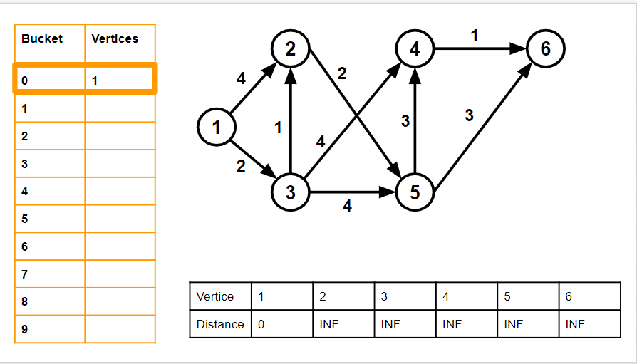
This is our example graph:
2. We can see it satisfies all properties. All edge weights are integers, and they are <=4.
We initialise the distance array (shown in the bottom as a black-bordered table), with all values infinity. 1 is our source. We keep the distance of the source as 0. The buckets table (shown as an orange-bordered table on the left) is initialised with all buckets empty, except the 0 bucket, which is filled with source vertex(1).
We have only shown 9 buckets here for simplicity. In actual implementations - there should be V*C = 6*4 = 24 buckets.
The time complexity of this algorithm is O(E+VC). We go through all the edges once (E), and we go through the entire buckets array once (V*C). The space complexity is O(VC) - the space needed for the buckets array.
Let's go through the algorithm now.
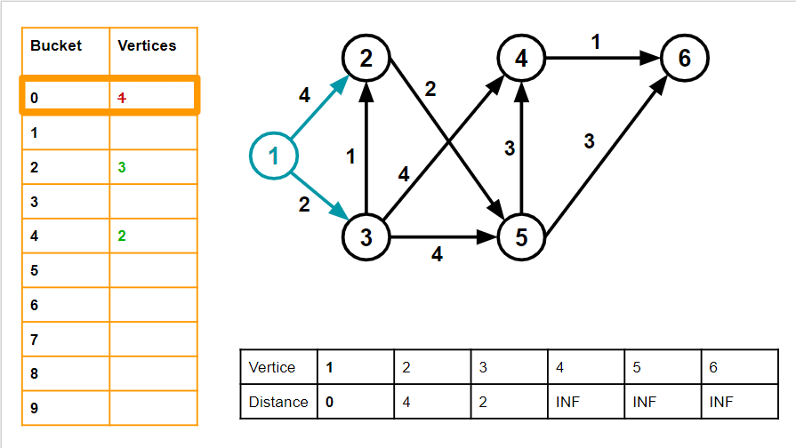
3. Our first minimum vertex (after EXTRACT MIN) is 1.
We go through the neighbours of 1– 2 and 3. Their distances are initially at Infinity. v=1.
For 2 , w = 4. dist[v] + w = 4, which is less than Infinity. So we move 2 into bucket number 4, and change dist[2] to 4 For 3, w =2. dist[v] + w = 2, which is less than infinity. So we move 3 into bucket number 2, and change dist[3] to 2 We remove 1 from its bucket
3. We advance the bucket pointer (the thick orange box) forward until we get a non-empty bucket
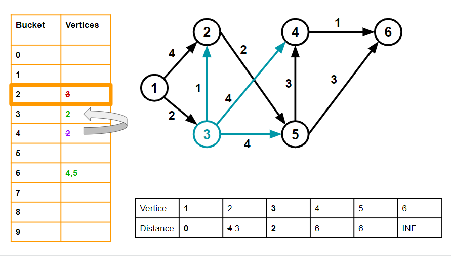
We come to vertice 3, v =3 and dist[v] = 2 We go through all it's neighbours.
For 2, w= 1 and dist[2] = 4. dist[v] +w = 2+1 = 3, which is < 4. So, we move 2 from bucket 4 to bucket 3 and set dist[2] as 3.
Similarly, for vertices 4 and 5, they are added to bucket number 6, and their distances are set to 6. We delete vertex 3 from its bucket
4. We again advance the bucket pointer forward until we arrive at a non-empty bucket.
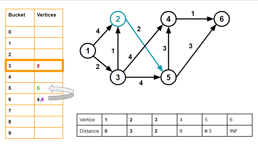
We arrive at bucket 3, with vertex 2. v=2, and dist[2] = 3. We go through all its neighbours. For vertex 5, w = 2 and dist[5] = 6. dist[v]+w =5, which is < 6. So we move vertex 5 from bucket 6 to bucket 5 and set dist[5] as 6.
We delete vertex 2 from its bucket
5.We advance the bucket pointer until we arrive at a non-empty bucket.
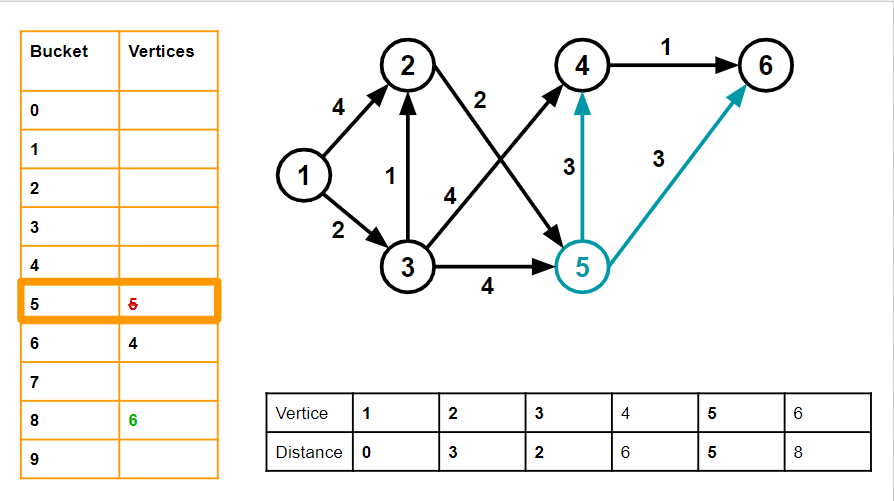
We arrive at bucket number 5, with vertex number 5. v=5, and dist[v] = 5. We go through all its neighbours.
For vertex 4, w = 3 and dist[4] = 6. dist[v]+3 = 8, which is > 8, so we let 4 remain unchanged.
Vertex 6 gets added to bucket 8, as we saw before, and its distance is set to 8. We delete vertex 5 from its bucket.
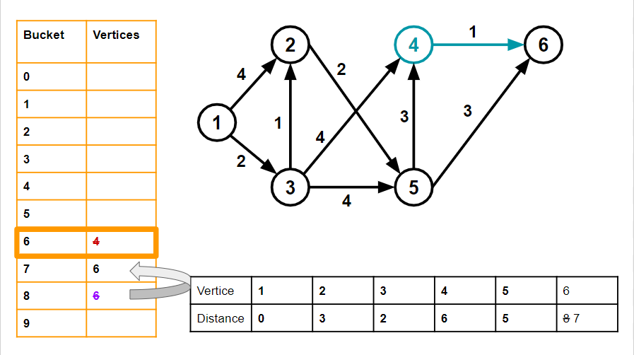
6. Advancing the bucket pointer, we arrive at bucket 6 and vertex 4
v=4, dist[v] = 6 4 has one neighbour 6. w for 6 is 1, and dist[6] is 8.
dist[v] + w = 7 ,which is < 8. So we move 6 from bucket 8 to bucket 7 and set dist[6] to 7. We delete 4 from its bucket.
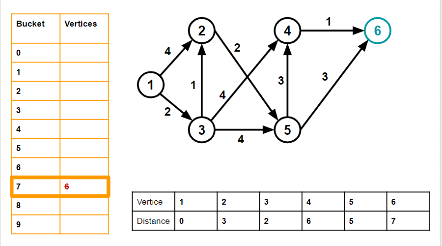
7. We advance the pointer until we reach bucket 7 and vertex 6. Vertex 6 has no neighbours, so we simply delete it from its bucket and move on.
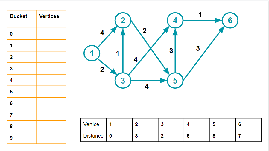
8. We iterate through the whole array (up till bucket 24, not 9 - 9 is shown here simply for representation, in reality, there will be 24 buckets), and we find no more empty buckets. Thus, our task is complete - and the dist table gives the shortest distance from Source (1) to each of the nodes.
Now, let's go straight into the code.
Implementation
C++
#include <iostream>
#include <vector>
#include <unordered_set>
using namespace std;

// This class represents a graph using adjacency list representation
class Graph {
  public:
    int V;         // no of vertices
    // adjacency list of the graph. adj[u] contains the list of pairs (v, w)
    // where
    //  v is a neighbour of u and w is the weight of the edge (u, v)
    vector<vector<pair<int, int>>> adj;
    Graph(int v) { // constructor
        V = v;
        // creates an adjacency list of size V+1, so that our vertices are
        // 1-indexed
        adj = vector<vector<pair<int, int>>>(V + 1);
    }
    // adds an edge from u to v, with weight w
    void addEdge(int u, int v, int w) { adj[u].push_back({v, w}); }
};
// Executes Dial's algorithm on the Graph g, and prints the shortest path
// from S to all other vertices. C is the maximum weight of any edge in the
// graph
void dialsAlgorithm(Graph g, int C, int S) {
    // The maximum number of buckets possible
    int maxBuckets = C * g.V;

    // buckets[i] stores all vertices that have a distance of i from S
    vector<unordered_set<int>> buckets(maxBuckets);

    // dist[i] stores the shortest distance from S to i
    //Initially, all distances are infinity or INT_MAX here.
    vector<int> dist(g.V + 1, INT_MAX);

    // initially, S is at distance 0 from itself
    dist[S] = 0;
    buckets[0].insert(S);

    // The current bucket that we are at in the algorithm
    int bucketPointer = 0;
    while (true) {
        // iterate through the buckets until we find a non-empty bucket, or run
        // out of buckets
        while (bucketPointer < maxBuckets && buckets[bucketPointer].empty()) {
            bucketPointer++;
        }

        // if we ran out of buckets, then we are done
        if (bucketPointer >= maxBuckets)
            break;

        // otherwise, we have found a non-empty bucket, and we will process it
        // We can choose any vertex. We will choose the first one.
        int v = *buckets[bucketPointer].begin();

        // remove v from the bucket, as we won't need it again.
        buckets[bucketPointer].erase(v);

        // iterate through all the neighbours of v
        for (pair<int, int> neiPair : g.adj[v]) {

            int nei = neiPair.first; // the neighbour
            int w = neiPair.second;  // the weight of the edge (v, nei)

            int altDist = dist[v] + w; // the distance from S to nei if we
                                       // travelled through v

            int currentDist = dist[nei]; // the current distance from S to nei

            // if we can improve the distance to nei by going through v, then we
            // will do so
            if (altDist < currentDist) {
                // if nei is not at infinity, it must be in some bucket. We will
                // remove it from that bucket
                if (currentDist != INT_MAX) {
                    buckets[currentDist].erase(nei);
                }

                // insert nei into the bucket that corresponds to its new
                // distance
                buckets[altDist].insert(nei);

                // update the distance to nei
                dist[nei] = altDist;
            }
        }
    }

    // print the shortest distances from S to all other vertices
    for (int i = 1; i <= g.V; i++) {
        cout << i << " ";
    }
    cout << endl;
    for (int i = 1; i <= g.V; i++) {
        cout << dist[i] << " ";
    }
    // And, we are done!
}
int main() {
    Graph g(6);
    g.addEdge(1, 3, 2);
    g.addEdge(1, 2, 4);
    g.addEdge(2, 5, 2);
    g.addEdge(3, 2, 1);
    g.addEdge(3, 4, 4);
    g.addEdge(3, 5, 4);
    g.addEdge(4, 6, 1);
    g.addEdge(5, 4, 3);
    g.addEdge(5, 6, 3);
    dialsAlgorithm(g, 4, 1);
    return 0;
}
You can also try this code with Online C++ Compiler
import javafx.util.Pair; //this class is not present in all version of Java, make sure it is present or the code won't run.
                                   // Coding Ninjas Studio Java Online Compiler has it.

import java.util.ArrayList;
import java.util.HashSet;

public class Solution{

    // This class represents a graph using adjacency list representation
    static class Graph {

        //The no. of vertices in the graph.
        public int V;

        // adjacency list of the graph. adj[u] contains the list of pairs (v, w)
        // where
        //  v is a neighbour of u and w is the weight of the edge (u, v)
        public ArrayList<ArrayList<Pair<Integer, Integer>>> adj;

        //Constructor
        public Graph(int V) {

            this.V = V;
            // creates an adjacency list of size V+1, so that our vertices are
            // 1-indexed
            adj = new ArrayList<>(V + 1);

            //We add empty ArrayLists so that we can access elements by index
            //right away, without having to add them later.
            for (int i = 0; i < V + 1; i++) {
                adj.add(new ArrayList<>());
            }
        }

        // adds an edge from u to v, with weight w
        public void addEdge(int u, int v, int w) {
            adj.get(u).add(new Pair<>(v, w));
        }
    }

    // Executes Dial's algorithm on the Graph g, and prints the shortest path
    // from S to all other vertices. C is the maximum weight of any edge in the
    // graph
    static void dialsAlgorithm(Graph g, int C, int S) {
        // The maximum number of buckets possible
        int maxBuckets = g.V * C;

        // buckets[i] stores all vertices that have a distance of i from S
        ArrayList<HashSet<Integer>> buckets = new ArrayList<>(maxBuckets);

        // Initialise buckets with empty sets, so we can access elements immediately.
        for (int i = 0; i < maxBuckets; i++) {
            buckets.add(new HashSet<Integer>());
        }

        //dist[i] stores the shortest distance of i from S
        ArrayList<Integer> dist = new ArrayList<>(g.V + 1);

        //Initialise dist with all values Infinity, or Integer.MAX_VALUE here
        for (int i = 0; i < g.V + 1; i++) {
            dist.add(Integer.MAX_VALUE);
        }

        //Initially, S it at distance 0 from itself.
        dist.set(S, 0);
        buckets.get(0).add(S);

        // The current bucket that we are at in the algorithm
        int bucketPointer = 0;

        while (true) {
            // iterate through the buckets until we find a non-empty bucket, or run
            // out of buckets
            while (bucketPointer < maxBuckets && buckets.get(bucketPointer).isEmpty()) {
                bucketPointer++;
            }
            // if we ran out of buckets, then we are done
            if (bucketPointer >= maxBuckets) break;

            // otherwise, we have found a non-empty bucket, and we will process it
            // We can choose any vertex. We will choose the first one.
            int v = buckets.get(bucketPointer).iterator().next();

            // remove v from the bucket, as we won't need it again.
            buckets.get(bucketPointer).remove(v);

            // iterate through all the neighbours of v
            for (Pair<Integer, Integer> pair : g.adj.get(v)) {
                int nei = pair.getKey(); // the neighbour
                int w = pair.getValue(); // the weight of the edge (v,nei)

                int altDist = dist.get(v) + w; // the distance from S to nei, if
                                               // travelled through v

                int currentDist = dist.get(nei); // the current distance from S to nei

                // if we can improve the distance to nei by going through v, then we
                // will do so
                if (altDist < currentDist) {
                    // if nei is not at infinity, it must be in some bucket. We will
                    // remove it from that bucket
                    if (currentDist != Integer.MAX_VALUE) {
                        buckets.get(currentDist).remove(nei);
                    }
                    // insert nei into the bucket that corresponds to its new
                    // distance
                    buckets.get(altDist).add(nei);

                    // update the distance to nei
                    dist.set(nei, altDist);
                }
            }
        }

        // print the shortest distances from S to all other vertices
        for (int i = 1; i <= g.V; i++) {
            System.out.print(i + " ");
        }
        System.out.println();
        for (int i = 1; i <= g.V; i++) {
            System.out.print(dist.get(i) + " ");
        }
        // And, we are done!
    }

    public static void main(String[] args) {
        Graph g = new Graph(6);
        g.addEdge(1, 3, 2);
        g.addEdge(1, 2, 4);
        g.addEdge(2, 5, 2);
        g.addEdge(3, 2, 1);
        g.addEdge(3, 4, 4);
        g.addEdge(3, 5, 4);
        g.addEdge(4, 6, 1);
        g.addEdge(5, 4, 3);
        g.addEdge(5, 6, 3);
        dialsAlgorithm(g, 4, 1);
    }
}
You can also try this code with Online Java Compiler
We can see from both the C++ and Java code that the following data structures are used:
An adjacency list containing E edges
A buckets array containing V*C buckets.
A dist array containing distances of V vertices
As the adjacency list is part of the input, we don't count it while we are deciding the space complexity.
For the other 2, the space complexity is O(V+V*C), which will simply be O(VC)
Time Complexity
From the code, we can see that we have two loops - the outer while loop, and the inner for loop (that iterates over neighbours)
For the outer while loop, the condition is true. However, we break out of it when bucketPointer goes past the value of maxBuckets. So, the outer while loop runs maxBuckets times, which is V*C
The inner for loop that iterates over neighbours - will go through all the edges. It won't go through all E edges every time, so we won't multiply over here. In total, E edges will be covered, so we will simply add.
Let's look at a few of the important applications of the Dijkstra algorithm:
1. Shortest Path Routing: Dijkstra's algorithm is widely used in network routing protocols to find the shortest path between two nodes in a graph. It is particularly useful in transportation networks, where it can be applied to find the shortest route between two locations considering factors like distance, time, or cost. For example, GPS navigation systems and mapping applications often use Dijkstra's algorithm to provide the optimal route for drivers.
2. Network Optimization: Dijkstra's algorithm plays a crucial role in optimizing network flows and minimizing costs. It can be used to find the shortest path in weighted graphs, where the weights represent costs or capacities. This has applications in various domains, such as telecommunication networks, where it helps in finding the most efficient path for data transmission, or in supply chain management, where it can optimize the distribution of goods from suppliers to customers.
3. Resource Allocation: Dijkstra's algorithm can be applied to resource allocation problems, where the goal is to allocate limited resources efficiently. For example, in a manufacturing setting, Dijkstra's algorithm can be used to determine the optimal allocation of machines to minimize production time or cost. It can also be used in task scheduling, where it helps in assigning tasks to resources in a way that minimizes the total completion time.
4. Social Network Analysis: Dijkstra's algorithm is useful in analyzing social networks and finding the shortest paths between individuals. It can be employed to identify the most influential people in a network based on their connectivity and the shortest paths to reach them. This has applications in viral marketing, where companies leverage social networks to spread their message efficiently, or in recommender systems, where it helps in suggesting relevant connections or content to users.
5. Robotics and Path Planning: In robotics, Dijkstra's algorithm is used for path planning and navigation. It can help robots find the shortest or most efficient path from a starting point to a destination while avoiding obstacles. This is particularly important in autonomous vehicles, where Dijkstra's algorithm can be used to plan safe and optimal routes considering factors like road conditions, traffic, and regulations.
6. Bioinformatics: Dijkstra's algorithm has applications in bioinformatics, particularly in sequence alignment and phylogenetic tree construction. It can be used to find the shortest path between sequences or to construct evolutionary trees based on genetic or protein sequences. This helps in understanding evolutionary relationships and identifying similarities or differences between species.
Frequently Asked Questions
What is the time complexity of Prim's and Dijkstra?
The time complexity of Prim's and Dijkstra's algorithms can both be O(E+VlogV)O(E+VlogV) when implemented with a priority queue.
What is the time complexity of Floyd's algorithm?
The time complexity of Floyd's algorithm is O(V3), where V is the number of vertices, making it suitable for dense graphs.
Is Dijkstra BFS or DFS?
Dijkstra's algorithm is neither BFS nor DFS; it is a greedy algorithm that uses a priority queue to find the shortest path from a single source.
Conclusion
We took a look at Dial's algorithm - which is a modified form of Dijkstra's algorithm. We saw in which conditions we can use it, what its logic is, and how it works. We went through an example solution to make it clearer - and we coded it in 2 languages.
We hope you leave this article with a broader knowledge of graphs, Dijkstra, and shortest-path algorithms. We recommend that you explore our different articles on these topics as well, such as:


 8+ registered

