Do you think IIT Guwahati certified course can help you in your career?
Introduction
In this blog, we will be studying the theory behind eigenvectors and eigenvalues.
Once done with this, we will be moving on to implementing the same in Python.
Theory
Eigenvectors are unit vectors, which implies that their magnitude is equivalent to 1. They are column vectors.
Eigenvalues are coefficients of eigenvectors, instrumental in defining their length.
A non-zero vector (eigenvector) changes by at most a scalar factor (eigenvalue) when a linear transformation is applied to it. The eigenvector points in a direction in which it is stretched by the transformation. The eigenvalue represents the factor by which it is stretched.
Mathematics Behind
Definition: Let A be an nxn matrix. A scalar λ is called an eigenvalue of A if there is a non-zero vector v such that:-
A.v = λ.v
The vector v is called an eigenvector of A corresponding to λ.
Let us take an example to understand the above statement.
Suppose we have the following:-
v = [ 2 ] = eigenvector
[ 1 ]
A = [ 3 2 ] = n*n matrix
[ 3 -2]
λ = 4 = eigenvalue
Now, we have to show that Av=λv.
So, we compute Av:-
A.v = [ 3 2 ] [ 2 ]
[ 3 -2] [ 1 ]
= [ 3*2 + 2*1]
[3*2 + -2*1]
= [6 +2]
[6 - 2]
= [8] - (a)
[4]
λ.v = 4 [ 2 ]
[ 1 ]
= [8] - (b)
[4]
From (a) and (b), we get that:-
A.v = λ.v
Note: If λ is an eigenvalue of the A and v is an eigenvector belonging to λ, then any non-zero multiple of v will be an eigenvector.
Now we know that A.v= λ.v . This gives us the following :
A.v = λ.v
A( m.v)
= m (A.v)
= m.λ.v
= λ (m.v)
Computation
Now, let us look at how to compute the eigenvalues and, in turn, compute the corresponding eigenvectors for a given matrix.
Let us assume we have an n*n matrix A and a scalar λ. Then it is essential to keep the following steps in mind for computing the eigenvalues and their corresponding eigenvectors:
Step 1: Multiply an n*n identity matrix by the scalar.
Step 2: Subtract the identity matrix multiple from the matrix.
Step 3: Find the determinant of the matrix and the difference.
Step 4 : Solve for the values of λ that satisfy the below equation :
det ( A - λI ) = 0
Step 5: Solve for the corresponding vector to each λ.
Let us take an example and compute the eigenvalues and the corresponding eigenvectors.
A = [ 7 3 ]
[ 3 -1 ]
(i) Firstly, we compute the identity matrix multiplied by the scalar.
λ.I = λ [ 1 0 ]
[ 0 1 ]
= [ λ 0 ]
[ 0 λ ]
(ii) Secondly, we subtract the identity matrix multiple from the matrix.
A - λ.I
= [ 7 3 ] - [ λ 0 ]
[ 3 -1 ] [ 0 λ ]
= [ 7-λ 3]
[ 3 -1-λ ]
(iii) Thirdly, let us find the determinant of the resultant matrix.
det ( 7-λ 3 )
( 3 -1-λ )
= (7-λ) (-1 - λ) -3(3)
= -7 -7λ + λ + λ2 -9
= λ2 -6λ - 16
(iv) Fourthly, let us compute the eigenvalues.
λ2 -6λ - 16
= λ2 -8λ + 2λ -16
= λ(λ -8) + 2(λ -8)
= (λ-8) (λ +2)
λ = 8 and λ=-2
(v) Lastly, let us find the corresponding eigenvectors.
For λ = 8, we get:-
B = [ 7-8 3 ]
[ 3 -1-8]
= [ -1 3 ]
[ 3 -9 ]
Now, we will solve for B.x = 0
[ -1 3 ] * [x1] = [0]
[ 3 -9 ] [x2] [0]
-x1 +3x2 = 0
3x1 -9x2 = 0
If we reduce the equations, both equations are the same. So, let us
take either and solve for x1 and x2 by cross shifting coefficients.
We get:-
-x1 +3x2 = 0
3x2= x1
x2/1 = x1/3
So we get that x2=1 and x1=3.
So, we get the eigenvector as [3] for λ=8.
[1]
Similarly, we can solve for λ= -2.
For λ=-2, we get :-
C = [ 7+2 3 ]
[ 3 -1+2]
= [ 9 3 ]
[ 3 1 ]
Now, we will solve for C.x = 0
[ 9 3 ] * [x1] = [0]
[ 3 1 ] [x2] [0]
9x1 +3x2 = 0
3x1 +x2 = 0
If we reduce the equations, both equations are the same. So, let us
take either and solve for x1 and x2 by cross shifting coefficients.
We get:-
3x1 +x2 = 0
3x1= -x2
x1/1 = x2/-3
So we get that x2=-3 and x1=1.
So, we get the eigenvector as [1] for λ=-2.
[-3]
Hence, we have computed the eigenvalues and the corresponding eigenvectors.
Implementation
Now, we will be going through the implementation of computing eigenvalues and eigenvectors using Python.
We will be using the same example used above to cross-verify the results. This would make understanding easier too.
Firstly, we would import the necessary libraries:
(i) NumPy - for constructing matrix.
(ii) eig - for computing eigenvalues and eigenvectors.
import numpy as np
from numpy import array
from numpy.linalg import eig
Now, we would be moving on to the computation.
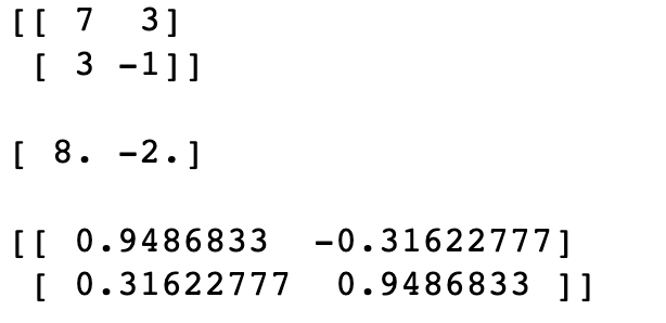
# define matrix
A = array([[7, 3], [3, -1]])
#printing matrix
print(A)
# calculating eigendecomposition
values, vectors = eig(A)
print(" ")
#printing eigenvalues
print((values))
print(" ")
#printing eigenvectors
print(vectors)
Output
In the above output, we notice that we've got the eigenvalues as 8 and -2. Also, we see that eigenvectors are normalized to unit length automatically.
Frequently Asked Questions
Q1. What is the difference between eigenvector and eigenvalue?
Eigenvectors are unit vectors, which implies that their magnitude is equivalent to 1, whereas Eigenvalues are coefficients of eigenvectors, instrumental in defining their length.
Q2. What is the equation to define the relationship between eigenvector and eigenvalue?
The equation is:- A.v = λ.v
where:-
A = n*n matrix
v = eigenvector
λ = eigenvalue
Key Takeaways
Congratulations on making it this far. This blog discussed a fundamental overview of Eigenvectors and Eigenvalues !!
We learned about computing eigenvectors and eigenvalues mathematically and their implementation in Python using a few essential libraries.
If you are preparing for the upcoming Campus Placements, don’t worry. Coding Ninjas has your back. Visit this link for a carefully crafted and designed course on-campus placements and interview preparation.


 9+ registered

