Get a skill gap analysis, personalised roadmap, and AI-powered resume optimisation.
Introduction
FP Growth stands tall in data mining as a powerful approach to identifying important patterns in large databases. As data keeps growing, old methods like Apriori become slow and difficult. FP Growth in Data Mining is a game changer that helps in finding important information from complex data.
In this article, we will study the working of FP algorithms in detail, along with their advantages and disadvantages.
FP Growth Algorithm
FP growth is a popular data Mining Algorithm used to find repeating patterns in big sets of data. It is faster than the older Apriori method as it does not waste time repeatedly analysing the same data set.
Han-in gave the FP (Frequent Pattern) algorithm. The algorithm does not need a lot of memory. It creates a tree called the FP (Frequent Pattern) tree to store the data capacity, and hence it can work quickly with large amounts of data.
The FP growth algorithm gives better results than Eclat and Relim and is used in many industries like market basket analysis, customer behavior modelling, and recommendation systems.
Working of FP Growth in Data Mining
The working of the FP algorithm in Data Mining can be understood with the steps below.
The algorithm first examines the dataset to see how often each item appears. It puts the most common items at the top of the list to further add them to the FP tree.
The items are sorted based on how frequent they are. Less common items are ignored or removed to make things faster.
After arranging the common items and counting the number of times they appear in the data, the algorithm constructs a special tree called the FP tree to represent the data compactly.
Once we have the FP tree, the FP algorithm can easily find and list all the common combinations of items in the data. Thus identifying patterns that appear most frequently in the data becomes easier.
Finally, the algorithm creates association rules by processing the frequent itemsets. These rules show the interesting connections between the different items in the dataset.
The FP tree is an important data structure used in FP Growth Data Mining. It represents the common patterns in the input data very efficiently. The key components of the FP tree are:
Root Node: The root node is the base or starting point of the FP tree. It does not represent any items but holds the links to the first nodes of each item.
Item Node: Each item in the dataset gets its own node. This node stores the name of the item and its frequency count in the dataset.
Header Table: The header table contains a list of distinct items in the dataset and their counts. The table records where the nodes are in the FP tree.
Child Node: If two items appear together in the same transaction, they become connected like friends. So each item node has child nodes representing items that commonly co-occur with it.
Node Link: Node link is a pointer that helps find the first node of each item in the FP tree. The pointer is useful when exploring patterns related to specific items.
The FP tree is constructed by analysing the input dataset and adding each transaction into the FP tree, one by one. For each transaction, we arrange the items in descending order of the count of how often they appear in the dataset and then insert them into the tree in that order. If the item already exists in the tree, the count is updated, and a new branch is created from the existing node. If an item is new, a new node is created for that item, and a new branch is added to the tree to represent this transaction in the tree.
Han's Algorithm
Let us understand Han's Algorithm with the help of an example. Consider the dataset as given below.
Transaction ID
Items
T1
{P, K, M, L, O, H}
T2
{D, P, K, L, O, H}
T3
{A, P, K, M}
T4
{C, K, M, U, H}
T5
{C, P, I, K, O, O}
In the above dataset, each letter represents an item. The frequency count of each item is defined in the table below.
Item
Frequency
A
1
C
2
D
1
H
3
I
1
K
5
L
2
M
3
O
4
P
4
U
1
Let’s assume we have a minimum support of 3, which means we want to find items that appear 3 times in the dataset.
After checking the data, it is observed that there are many items, each with its count. Hence we only keep the things with a count of 3 or more: H, K, M, O, P.
Next, the transactions in the dataset are rearranged. For each transaction, we will remove items that appear less than 3 times and sort the remaining items in descending order of their frequency.
Transaction ID
Items
Re-arranged Item sets
T1
{P, K, M, L, O, H}
{K, P, M, O, H}
T2
{D, P, K, L, O, H}
{K, P, O, H}
T3
{A, P, K, M}
{K, P, M}
T4
{C, K, M, U, H}
{K, M, H}
T5
{C, P, I, K, O, O}
{K, P, O}
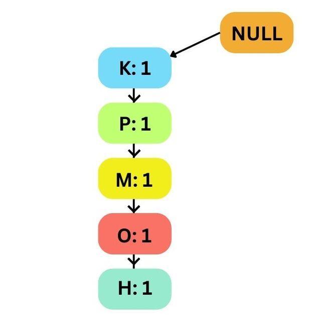
First Transaction T1
All items are linked together, and each item has a support count of 1.
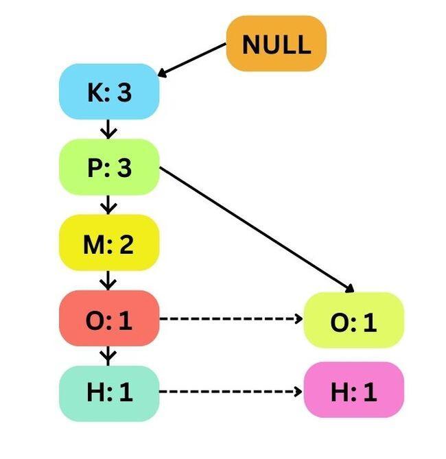
Second Transaction T2
Here the K and P appear again, so their support count is updated to 2. Since there’s no direct link from P to O, we create a new branch for O and H with support count 1.
Third Transaction T3
Now that K and P have appeared three times, so their support count is increased to 3, and M appears twice, so its support count becomes 2.
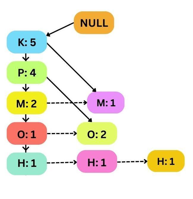
Fourth Transaction T4 and Fifth Transaction T5
After inserting the last two transactions, the FP tree is updated with the new support counts.
Next, we will create a “Conditional Pattern Base” for each frequent item. The conditional Pattern Base is like a list of paths in the FP tree that end with the specific frequent item we are interested in. For example, for item O, the paths {K, P, M} and {K, P} in the FP tree will be part of its conditional Pattern Base. Hence the conditional Pattern Base for the above dataset is as follows:
Items
Conditional Pattern Base
H
{{K, P, M, O: 1}, {K, P, O: 1}, {K, M: 1}}
O
{{K, E, M: 1}, {K, E: 2}
M
{{K,E: 2}, {K: 1}}
P
{K: 4}
K
Next we will be building the Conditional Frequent pattern Tree for each item, and find the common elements in their related paths. The support count is calculated by adding the support counts of these paths.
Items
Conditional Pattern Base
Conditional Frequent Pattern Tree
H
{{K, P, M, O: 1}, {K, P, O: 1}, {K, M: 1}}
{K: 3}
O
{{K, P, M: 1}, {K, P: 2}
{K, : 3}
M
{{K,P: 2}, {K: 1}}
{K: 3}
P
{K: 4}
{K: 4}
K
Using the conditional FP tree, as shown above, we can create the frequent itemsets as listed in the table below:
Items
Frequent Pattern Generated
H
{K, Y: 3}
O
{{K, O: 3}, {P, O: 3}, {P, K, O: 3}}
M
{K, M: 3}
P
{P, K: 4}
K
FP Algorithm Vs Apriori Algorithm
The difference between FP Algorithm Vs Apriori Algorithm are as follows:
FP Algorithm
Apriori Algorithm
FP growth uses a special tree called the FP tree to find frequent itemsets in one go.
The Apriori algorithm iteratively mines the common itemsets step by step.
FP Growth analyses the database only two times to build an FP tree to find patterns.
The Apriori algorithm needs to scan the database many times to find the common itemsets.
FP Growth is faster because it uses smart data compression and creates itemsets more efficiently.
Apriori is slower because it scans the database many times to generate the itemsets, which takes more time.
FP Growth uses less memory.
Apritori takes more memory.
FP Growth works well on large datasets.
Apriori does not give good results with big datasets.
Advantages of FP Growth in Data Mining
The advantages of FP Growth in Data Mining are:
FP growth is quicker and requires less computer memory than similar algorithms like Apriori. It can handle big datasets with many items efficiently.
When dealing with large datasets, FP growth performs well. It handles increasing data size and complexity without slowing down.
The algorithm is good at handling data that may have some noisy items. It focuses only on finding common patterns and ignores the rest.
FP growth can easily split and be processed across many computers or processors at the same time. This makes it very suitable for modern computing environments.
Disadvantages of FP Growth in Data Mining
The disadvantages of FP Growth in Data Mining are:
FP growth is usually good with memory usage, but with the increase in the size of data, lots of memory is required for the effective working of the algorithm. When the dataset contains more distinct items, the size of the FP also increases, resulting in more memory usage.
FP growth can be difficult to understand and put into practice as compared to some other ways of finding common itemsets in data.
When the minimum support is set too high, FP growth can take a long time to find patterns as it needs to search through long branches in the data.
FP growth is good at finding common patterns, but it's not the best choice if rare patterns are to be identified.
Frequently Asked Questions
What is the FP Growth in Data Mining?
FP growth is a popular data Mining Algorithm used to find repeating patterns in big sets of data. It is faster than the older Apriori method as it does not waste time analyzing the same data set repeatedly. The algorithm creates a tree called the FP (Frequent Pattern) tree to store the data capacity, and hence it can work quickly with large amounts of data.
What is an FP tree?
The FP tree is an important data structure used in FP Growth Data Mining. It represents the common patterns in the input data very efficiently. The FP tree is constructed by analyzing the input dataset and adding each transaction into the FP tree, one by one.
What are the differences between FP Growth and Apriori algorithm?
The key difference between FP and Apriori algorithms is that FP growth uses a special tree called the FP tree to find frequent itemsets in one go. The Apriori algorithm iteratively mines the common itemsets step by step.
Mention some advantages of FP Growth in Data Mining?
The key advantages of FP Growth in Data Mining is that FP growth is quicker and requires less computer memory than similar algorithms like Apriori. It can handle big datasets with many items efficiently. When dealing with large datasets, FP growth performs well. It handles increasing data size and complexity without slowing down.
Conclusion
Kudos on finishing this article! We have discussed how efficiently FP Growth in Data Mining can be used to identify patterns in big datasets.
We hope this blog has helped you enhance your knowledge of FP Growth in Data Mining.
Keep learning! We suggest you read some of our other articles related to Data Mining:
But suppose you are just a beginner and are looking for questions from tech giants like Amazon, Microsoft, Uber, etc. For placement preparations, you must look at the problems,interview experiences, andinterview bundles.


 9+ registered

