Gated Recurrent Units (GRUs)

Introduction

Neural Networks have gained a lot of value due to their ability to solve many problems with great accuracy. Much research and work are done to make these neural networks better, faster, and more accurate. Gated recurrent units (GRU) are a recent development in recurrent neural networks. Let us learn more about GRUs in detail.

Background: RNN and LSTM

Recurrent Neural Networks (RNN)

RNN is an artificial neural network where the nodes form a sequence. It uses the output from the previous step and the current input to get the output of the current node. It has an internal memory that saves all the information. It uses the same functions on all the inputs and is called ‘recurrent’.

RNN Cell

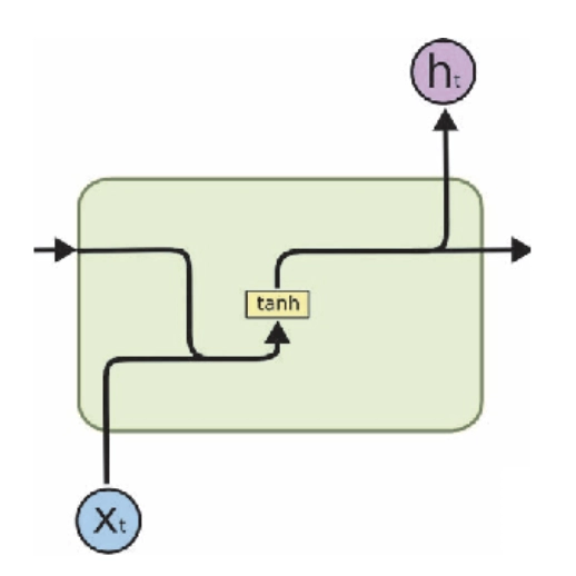
As RNN process the previous inputs, it performs well on our sequential input. But due to this repeated calculation on all the inputs, the problem of ‘vanishing gradient’ or ‘exploding gradient’ arises. It fails to handle “long-term dependencies” as the inputs stored a long time ago can vanish and become useless.

RNN Architecture:

1. Input Layer:
   Takes in sequential data (e.g., words, time steps) one element at a time.
2. Hidden Layer (Recurrent Cell):
   Each cell receives the current input and the hidden state from the previous time step. It applies the same function repeatedly across all time steps, enabling the model to retain context and learn patterns over sequences.
3. Output Layer:
   Produces the output for each time step, based on the current hidden state.

The ability of RNNs to “remember” past inputs allows them to learn time-dependent patterns and relationships within data. However, retaining this information accurately over longer sequences is challenging.

Limitations of RNNs

• Vanishing Gradient Problem:
  During backpropagation through time, gradients can shrink exponentially, making it difficult for the model to learn long-range dependencies.
• Exploding Gradients:
  In some cases, gradients may grow uncontrollably, destabilizing learning.
• Poor Long-Term Memory:
  As a result, RNNs struggle with tasks requiring memory of information seen many time steps earlier, limiting their effectiveness for longer sequences.

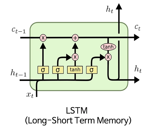
Long Short Term Memory (LSTM)

LSTM is a modified RNN. It stands for Long Short Term Memory. RNN has a single layer of tanh, while LSTM has three sigmoid gates and one tanh layer. The gates in LSTM decide the information to be sent to the next layer and the information that is to be rejected. The gates allow the gradients to flow unchanged without any calculation, solving the problem. 

LSTM Cell 

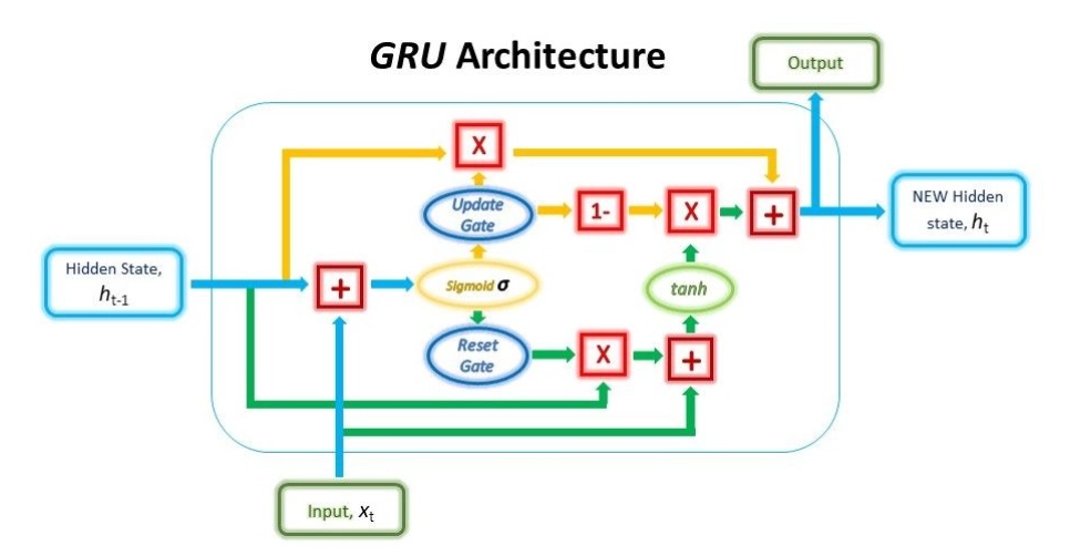
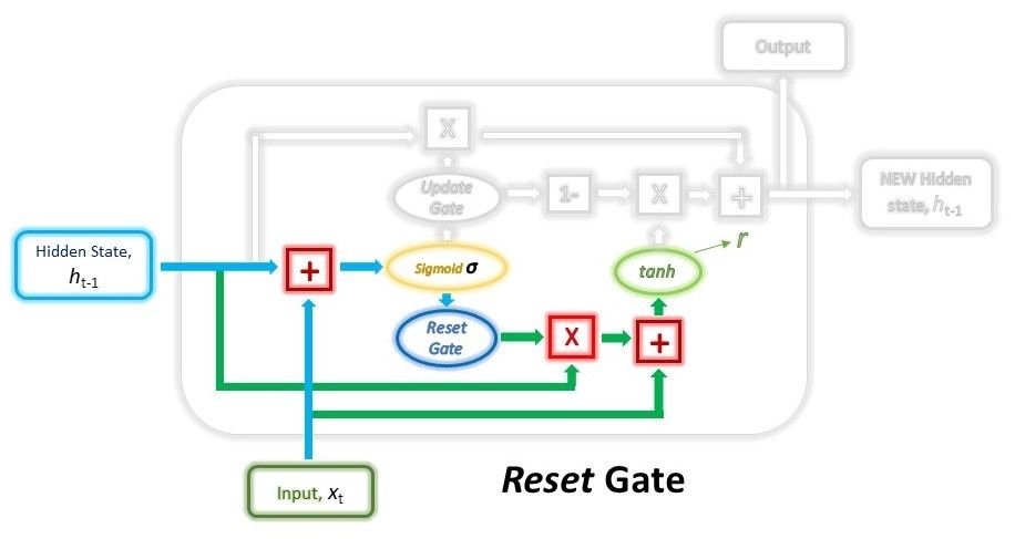
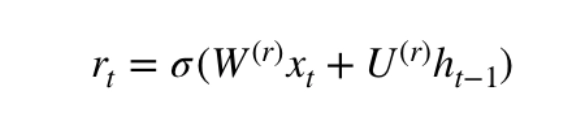
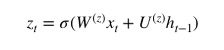
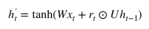
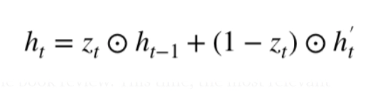
We used LSTM for a long time to solve the problem of vanishing gradients. GRU is a recent installment in this field that is similar to LSTM.

LSTM Gating Mechanism:

1. Input Gate:
   Controls how much of the new input should be written to the cell state. It filters relevant incoming information that should influence the future states.
2. Forget Gate:
   Decides what portion of the previous cell state should be discarded. It plays a key role in preventing irrelevant or outdated data from cluttering memory.
3. Output Gate:
   Determines which part of the cell state will be passed as the output and hidden state to the next time step or layer.

These gates allow LSTM networks to preserve important patterns over long sequences without losing valuable gradient flow during training.

Real-World Applications of LSTM:

• Sentiment Analysis:
  Captures context in user reviews or tweets to determine sentiment over a series of words.
• Speech Recognition:
  Maintains understanding of audio sequences, improving the accuracy of transcriptions.
• Machine Translation:
  Translates sentences by remembering context and structure over long input sequences.

Limitations of LSTM

While LSTMs offer significant improvements over traditional RNNs, especially in handling long-term dependencies, they come with several limitations that can impact performance and scalability.

• Computationally Heavy:
  LSTM networks are more complex than simple RNNs due to their multiple gating mechanisms—input, forget, and output gates. Each gate performs its own matrix operations, which increases the number of parameters and computational load. This makes LSTMs slower during both training and inference, especially for large datasets or real-time applications.
• High Memory and Longer Training Time:
  The added complexity in architecture means LSTMs require more memory to store parameters and intermediate states. As a result, training takes significantly longer compared to simpler architectures, and the model may require more data to generalize effectively.
• Difficulty with Very Long Sequences:
  Although LSTMs were designed to handle long-range dependencies, they can still struggle with very long sequences. Their ability to retain information gradually diminishes over extreme time steps, making them less effective in applications that require deep memory.
• Lack of Parallelization:
  Due to their sequential nature, where each time step relies on the output of the previous one, LSTMs cannot be fully parallelized during training. This limits their efficiency on modern hardware, especially GPUs, which are optimized for parallel operations.