Do you think IIT Guwahati certified course can help you in your career?
Introduction
Gaussian Elimination stands as a foundational and powerful method in linear algebra, offering a systematic approach to solving systems of linear equations. In this article, we will discuss Gaussian Elimination to Solve Linear Equations.
We all are aware of linear equations. It is a group of linear equations with various unknown factors. The unknown factors exist in multiple equations, and we need to solve a linear equation to find those unknown constants. One such method to solve a system of linear equations is Gaussian elimination.
Before proceeding further, let's first understand the concept of Gaussian elimination.
Let's explore how the gaussian elimination method helps us find the solutions to the linear equations.
Gaussian elimination
The gaussian elimination is an algorithm in linear algebra that lets you find the solutions to a linear system.
The central concept of this algorithm is to add multiples of one (smallest) equation to the others to remove a variable and to keep doing so until there is only one variable remaining. The value of this last variable is determined and then substituted back into the other equations to evaluate the different unknown values. Hence gaussian elimination method is a step‐by‐step elimination of the variables.
To apply gaussian elimination, you can algebraically operate on the columns and rows of a matrix in the given three ways:
You can interchange two rows.
You can multiply a row by any non-zero constant.
You can also add a row to another row to form an upper triangular matrix.
Augmented Matrix
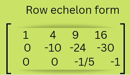
To find the values of the unknowns in gaussian elimination, we convert the augmented matrix into the row echelon form and carry out the backward substitution. This method, also known as row reduction, contains two steps: back substitution and forward elimination.
Row Echelon Form
All rows with at least one non-zero element are above all-zero rows.
Each row's leading coefficient(first non-zero element) should be one.
The matrix is in an upper triangular matrix.
Solving a linear system with an augmented matrix using Gaussian elimination is a structured, organized, and quite efficient method.
Gauss Elimination Method with Example
Gaussian Elimination, a fundamental technique in linear algebra, provides a systematic approach to solving systems of linear equations. Let's explore this method through an illustrative example.
Consider the system:
2x+y−z = 8 −3x−y+2z = -11 −2x+y+2z = -3
The goal is to transform this system into an equivalent, simpler system with a unique solution through a series of elementary row operations.
Step 1: Augmented Matrix
2 1 -1 | 8
-3 -1 2 | -11
-2 1 2 | -3
Step 2: Row Operations
R2=R2 + 3/2R1 R3= R3 + R1
2 1 -1 | 8
0 -½ ½| 1
0 2 1 | 5
Step 3: Row Operations
R3= R3 - 4R2
2 1 -1 | 8
0 -½ ½| 1
0 0 -1 | 1
Step 4: Back Substitution
z=−1
Substitute back into the second equation to find y:
-½y + ½(-1) = 1
Finally, substitute back into the first equation to find x:
2x+ 2 -1= 8
x=3
The solution to the system of linear equations is x=3, y=2, and z=-1. Gaussian Elimination has successfully transformed the system into a simplified form, revealing the unique solution to the given set of equations.
Gauss Elimination Problems
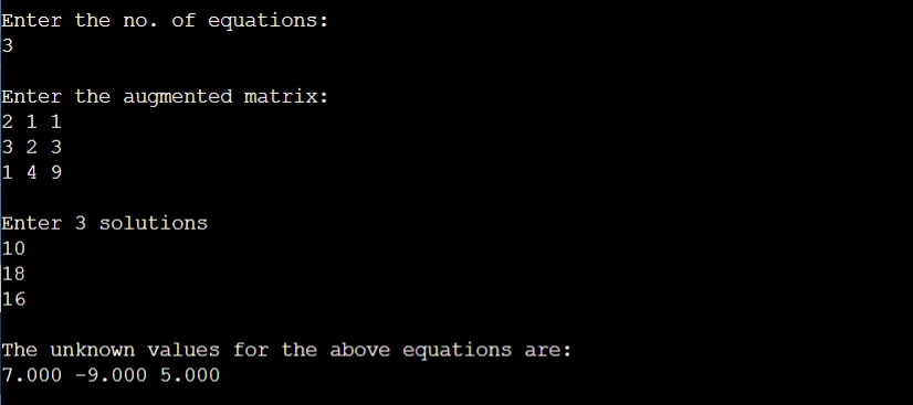
Find the unknown variables using the Gaussian elimination method for the given linear equations.
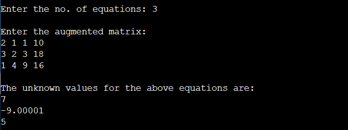
Input
Enter the no. of equations: 3
Enter the augmented matrix:
2 1 1 10
3 2 3 18
1 4 9 16
Output
The unknown values for the above equations are:
7
-9.00001
5
Explanation
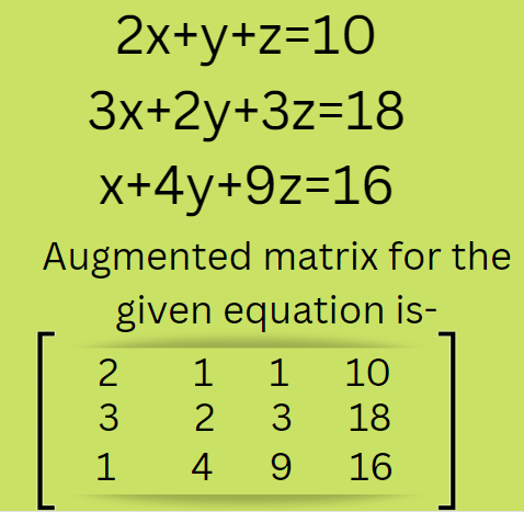
The given input forms the matrix having n rows and n+1 columns depending on the number of unknown constants(n). The input matrix represents the following equations-
2X + Y + Z = 10
3X + 2Y + 3Z = 18
X + 4Y + 9Z = 16
Algorithm
First, we will define the number of rows(n) and columns(n+1) or the number of equations.
The second step is to read the number of unknown variables(n).
Read augmented matrix of n X n+1 Size
For i = 0 to n

For j = 0 to n+1

Read matrix[i][j]

Next j

Next i
Transform Augmented Matrix (A) by performing the shifting operations and applying gaussian elimination to form an upper triangular matrix.
Applying Gauss Elimination on input matrix:
For i = 0 to n-1

If matrix[i][j] = 0

Print "Error"
Stop

End If

For j = i+1 to n

Ratio = matrix[j],i/matrix[i],i

For k = 0 to n+1

matrix[i][k] = matrix[j][k] - Ratio * matrix[i][k]

Next k
Next j
Next i
The next step is to obtain a solution by Back Substitution.
Xn = matrix[n],n+1/matrix[n],n

For i = n-1 to 1
Xi = matrix[i],n+1

For j = i+1 to n

Xi = Xi - matrix[i][j] * Xj

Next j

Xi = Xi/matrix[i],i
Next i
Now we can see the output in the console.
The implementation of the above algorithm is given below.
Implementation in C++
C++
C++
#include<iostream>
#include<math.h>

using namespace std;

int main() {
  int i, j, k, n;

  cout << "\nEnter the no. of equations: ";
  cin >> n;

  // Here size of the augmented matrix will be n*n+1
  float matrix[n][n + 1];

  /* we will store the n unknown constants of n equations in array 'result' */
  float result[n];

  cout << "\nEnter the augmented matrix: ";
  for (i = 0; i < n; i++) {
    for (j = 0; j < n + 1; j++) {
      cin >> matrix[i][j];
    }
  }

  for (i = 0; i < n; i++) {
    for (j = i + 1; j < n; j++) {
      if (abs(matrix[i][i]) < abs(matrix[j][i])) {
        for (k = 0; k < n + 1; k++) {

          /* we will swap the matrix[i][k] and matrix[j][k] to get the lowest element on top */
          matrix[i][k] = matrix[i][k] + matrix[j][k];
          matrix[j][k] = matrix[i][k] - matrix[j][k];
          matrix[i][k] = matrix[i][k] - matrix[j][k];
        }
      }
    }
  }

  /* Using Gaussian elimination to form upper triangular matrix */
  for (i = 0; i < n - 1; i++) {
    for (j = i + 1; j < n; j++) {
      float f = matrix[j][i] / matrix[i][i];
      for (k = 0; k < n + 1; k++) {
        matrix[j][k] = matrix[j][k] - f * matrix[i][k];
      }
    }
  }

  /* Using backward substitution to find the unknown values */
  for (i = n - 1; i >= 0; i--) {
    result[i] = matrix[i][n];

    for (j = i + 1; j < n; j++) {
      if (i != j) {
        result[i] = result[i] - matrix[i][j] * result[j];
      }
    }
    result[i] = result[i] / matrix[i][i];
  }

  cout << "\nThe unknown values for the above equations are:\n";
  for (i = 0; i < n; i++) {
    cout << result[i] << "\n";
  }
  return 0;
}
You can also try this code with Online C++ Compiler
The time complexity for the above code will be O(n)*(O(n)*O(n)) = O(n3) because for each pivot, we will traverse the part to its right for each row below it. Whereas the space complexity is O(n^2).
Implementation in Java
Java
Java
import java.util.Scanner;

public class Main
{
    public void solveMatrix(double[][] A, double[] B)
    {
        int N = B.length;
        for (int k = 0; k < N; k++)
        {
            /** find pivot row **/
            int max = k;
            for (int i = k + 1; i < N; i++)
                if (Math.abs(A[i][k]) > Math.abs(A[max][k]))
                    max = i;

            /** swap row in A matrix **/
            double[] temp = A[k];
            A[k] = A[max];
            A[max] = temp;

            /** swap corresponding values in constants matrix **/
            double t = B[k];
            B[k] = B[max];
            B[max] = t;

            /** pivot within A and B **/
            for (int i = k + 1; i < N; i++)
            {
                double factor = A[i][k] / A[k][k];
                B[i] -= factor * B[k];
                for (int j = k; j < N; j++)
                    A[i][j] -= factor * A[k][j];
            }
        }

        /* Using back substitution to find unknown variables*/
        double[] solution = new double[N];
        for (int i = N - 1; i >= 0; i--)
        {
            double sum = 0.0;
            for (int j = i + 1; j < N; j++)
                sum += A[i][j] * solution[j];
            solution[i] = (B[i] - sum) / A[i][i];
        }
        /** Print solution **/
        printSolution(solution);
    }

    /* function to print solution */
    public void printSolution(double[] sol)
    {
        int N = sol.length;
        System.out.println("\n The unknown values for the above equations are: ");
        for (int i = 0; i < N; i++)
            System.out.printf("%.3f ", sol[i]);
        System.out.println();
    }

    /** Main function **/
    public static void main (String[] args)
    {
        Scanner scan = new Scanner(System.in);
        /** Make an object of Main class **/
        Main ge = new Main();

        System.out.println("\nEnter the no. of equations:");
        int N = scan.nextInt();

        double[] B = new double[N];
        double[][] A = new double[N][N];

        System.out.println("\nEnter the augmented matrix:");
        for (int i = 0; i < N; i++)
            for (int j = 0; j < N; j++)
                A[i][j] = scan.nextDouble();

        System.out.println("\nEnter "+ N +" solutions");
        for (int i = 0; i < N; i++)
            B[i] = scan.nextDouble();
        ge.solveMatrix(A,B);
    }
}
You can also try this code with Online Java Compiler
The time complexity for the above code will be O(n)*(O(n)*O(n)) = O(n3) because for each pivot, we will traverse the part to its right for each row below it. Whereas the space complexity is O(n^2).
Implementation in Python
Python
Python
# Importing NumPy Library import numpy as np import sys
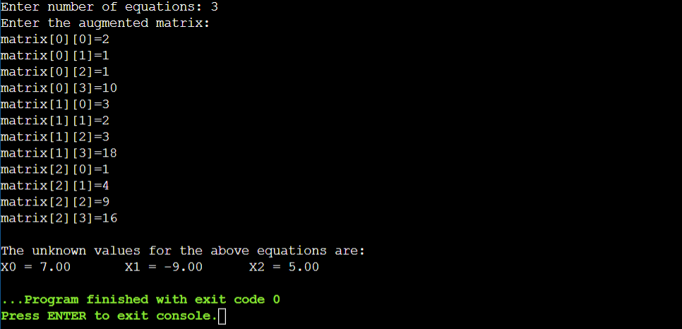
n = int(input('Enter number of equations: '))
# Making numpy array of n x n+1 size and initializing # to zero for storing augmented matrix matrix = np.zeros((n,n+1))
# Making numpy array of n size and initializing # to zero for storing solution vector x = np.zeros(n)
# Reading augmented matrix coefficients print('Enter the augmented matrix:') for i in range(n): for j in range(n+1): matrix[i][j] = float(input( 'matrix['+str(i)+']['+ str(j)+']='))
# Applying Gauss Elimination for i in range(n): if matrix[i][i] == 0.0: sys.exit('Error! division by zero detected!')
for j in range(i+1, n): ratio = matrix[j][i]/matrix[i][i]
for k in range(n+1): matrix[j][k] = matrix[j][k] - ratio * matrix[i][k]
# Back Substitution x[n-1] = matrix[n-1][n]/matrix[n-1][n-1]
for i in range(n-2,-1,-1): x[i] = matrix[i][n]
for j in range(i+1,n): x[i] = x[i] - matrix[i][j]*x[j]
x[i] = x[i]/matrix[i][i]
# Displaying solution print('\nThe unknown values for the above equations are:') for i in range(n): print('X%d = %0.2f' %(i,x[i]), end = '\t')
You can also try this code with Online Python Compiler
The time complexity for the above code will be O(n)*(O(n)*O(n)) = O(n3) because for each pivot, we will traverse the part to its right for each row below it.
Now it’s time for some frequently asked questions.
Frequently Asked Questions
What are the rules for Gaussian elimination?
The rules for Gaussian elimination is to perform elementary row operations: interchange rows, multiply a row by a non-zero constant, and add or subtract a multiple of one row from another.
Why is it called Gaussian elimination?
It is named after Carl Friedrich Gauss, it's a method for transforming a matrix to its row-echelon form.
What is Gaussian elimination method disadvantages?
Gaussian elimination method disadvantages are sensitivity to round-off errors and computational complexity for large systems.
Can you divide in Gaussian elimination?
Division is involved when scaling rows but not when performing basic row operations.
Conclusion
In the above article, we have learned to calculate the value of unknown variables in linear equations using the gaussian elimination method. We have discussed the approach using java, python, and CPP languages. To enhance your knowledge of gaussian algorithms, check out these articles-
Refer to our guided paths on Coding Ninjas Studio to learn more about DSA, Competitive Programming, JavaScript, System Design, etc. Enroll in our courses and refer to the mock test and problems available. Take a look at the interview experiences for placement preparations.


 9+ registered

