Gaussian Naive Bayes

Gaussian Naive Bayes

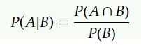
We've seen that the events(A1, A2,...) are in categories so far, but what about when an event is a continuous variable? If we suppose that event follows a specific distribution, the probability of likelihoods are calculated using the probability density function of that distribution.

sourceLink

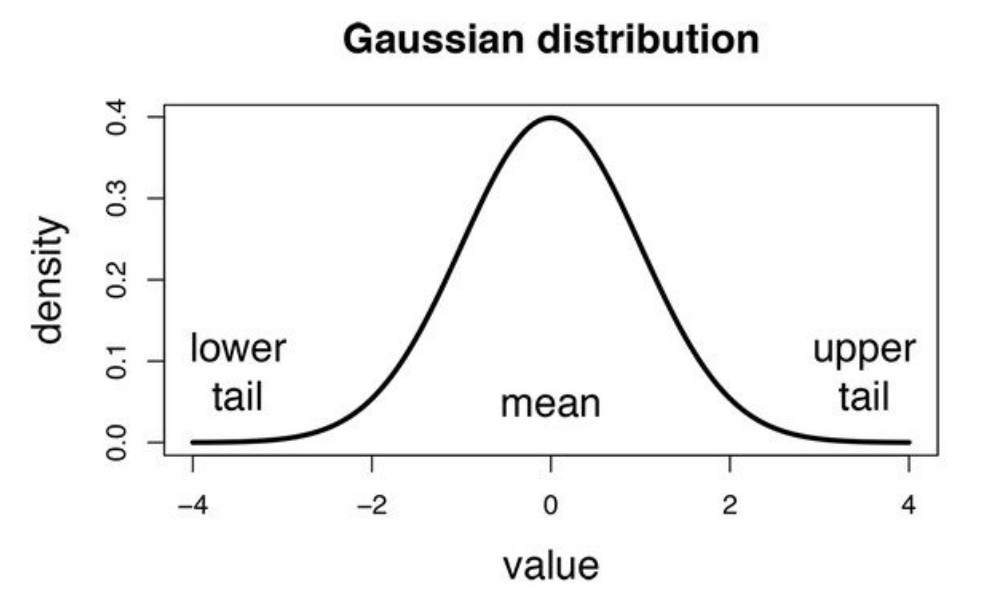
If we assume that events follow a Gaussian or normal distribution, we must use its probability density and call it Gaussian Naive Bayes.

For the Naive gaussian Bayes, we use the following form:

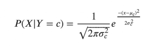
The variance and mean of the continuous variable X determined for a given class c of Y are σ and μ in the following formulas.

Let's use Python,, and Scikit Learn to implement Gaussian Naive Bayes in practice.

Implementation

%matplotlib inline

 
From sklearn.datasets import make_blobs, make_moons, make_regression, load_iris
from scipy.stats import multivariate_normal
import matplotlib.pyplot as plt
import numpy as np

 
# For the moment we only take a couple of features from the IRIS dataset for convenience of visualization 

 
iris = load_iris()
X = iris.data[:, 1:3]  
Y = iris.target

 
print X.shape
print Y.shape
plt.scatter(X[:,0],X[:,1])


 
#algorithm implementation.

 
class BayesClassifier:
    
    mu = None
    cov = None
    n_classes = None
    
    def __init__(self):
        a = None
    
    def pred(self,x):
        prob_vect = np.zeros(self.n_classes)
        
        for i in range(self.n_classes):
            
            
            mnormal = multivariate_normal(mean=bc.mu[i], cov=bc.cov[i])
            
            # We use uniform priors
            prior = 1./self.n_classes
            
            prob_vect[i] = prior*mnormal.pdf(x)
            sumatory = 0.
            for j in range(self.n_classes):
                mnormal = multivariate_normal(mean=bc.mu[j], cov=bc.cov[j])
                sumatory += prior*mnormal.pdf(x)
            prob_vect[i] = prob_vect[i]/sumatory
        return prob_vect
        
    def fit(self, X,y):
        self.mu = []
        self.cov = []
        
        self.n_classes = np.max(y)+1
        
        for i in range(self.n_classes):
            Xc = X[y==i]
            
            mu_c = np.mean(Xc, axis=0)
            self.mu.append(mu_c)
            
            cov_c = np.zeros((X.shape[1], X.shape[1]))
            for j in range( Xc.shape[0]):
                a = Xc[j].reshape((X.shape[1],1))
                b = Xc[j].reshape((1,X.shape[1]))
                cov_ci = np.multiply(a, b)
                cov_c = cov_c+cov_ci
            cov_c = cov_c/float(X.shape[0])
            self.cov.append(cov_c)
        self.mu = np.asarray(self.mu)
        self.cov = np.asarray(self.cov)

 
# Fit the classifier
bc = BayesClassifier()

 
bc.fit(X,Y)

You can also try this code with Online Python Compiler

Run Code

FAQs

1. Is Gaussian naive Bayes suitable for datasets with a large number of attributes??
   If the number of characteristics is enormous, the computation cost will be considerable, and the Curse of Dimensionality will apply.
    
2. What is the zero frequency phenomenon?
   The model is given a 0 (zero) probability if a category is not recorded in the training set but occurs in the test data set, resulting in an erroneous estimate.
    
3. What exactly does the word distribution signify?
   Distribution shows how values disperse in series and how frequently they appear in this series.
    
4. When is gaussian naive bayes used?
   It is more likely to be used when each class follows a Gaussian distribution.
    
5. What is a confusion matrix?
   A confusion matrix is a method for evaluating machine learning classification performance. It allows you to assess the performance of the classification model using a set of test data for which the true and false values are known.

Key Takeaways

There are several different  naive Bayes algorithms whose usability can be referred to here.