Gradient Descent Algorithm
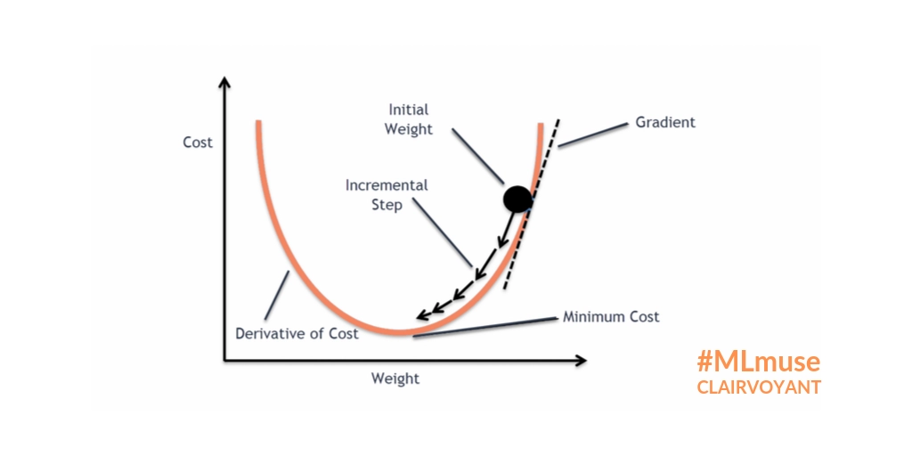
It is an iterative process that calculates the coordinates of the next point using gradient at the current point, multiples it(by a factor of learning rate) and subtracts the resultant from the current point. Thereby, completing one step. We are subtracting here as our goal is to minimize the function. Mathematically, the process of step calculation would look like this:

Here, pn+1 is the value of the new weight to be calculated pn is the value of the old weight. The parameter η is the learning rate here and has quite some influence on the model’s behavior(as seen earlier). η is then multiplied by the gradient at that particular point(calculated using derivative)
To learn more about how this equation is derived, feel free to check this post out.
Let’s try and implement the above algorithm into code.
Algorithm
# gradient function computes the derivative of the cost function
___________________________________________________________________
Procedure gradient_descent(start, gradient, learning_rate, max_iter, tol):
___________________________________________________________________
1. steps ← start, x ← start # variables initialization
2. for iterations = 1 to max_iter do
3. diff ← learning_rate*gradient(x) # computing the learning_rate*gradient
4. if abs(diff) < tol do # if the score is not going to improve
5. break
6. end if
7. x ← x - diff # x are the weights to be updated
8. return steps, x
9. end procedure
___________________________________________________________________
The function gradient_descent takes five parameters:
- start: It defines the starting point of the algorithm(usually initialized randomly).
- gradient: This function has to be pre-specified.
- learning_rate: This is the learning rate as we discussed above.
- max: This limits the maximum number of iterations that can take place.
- tolerance: To conditionally stop the function, we can assign a default value. In this case, it is 0.001.
Read about Batch Operating System here.
Types of Gradient Descent
In current machine learning and deep learning algorithms, there are three primary forms of gradient descent. The primary cause for these variances is computing efficiency. It boils down to the gradient's accuracy vs. the time it takes to compute the next step. With that said, let's have an overview of the three types of gradient descent, understand each type and go over their pros and cons.
Batch Gradient Descent
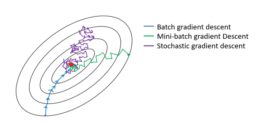
The most basic kind is Batch Gradient Descent. Within the training set, it estimates the error for each example. It changes the model parameters only when it has evaluated all of the training instances.
Advantages
- Using a fixed learning rate during training eliminates the risk of learning rate degradation.
- It calculates gradients in an impartial manner. The standard error is reduced as the number of examples increases.
Disadvantages
- It will take a long time to run through all of the examples, especially when dealing with massive datasets.
- Each learning step occurs after reviewing all examples, some of which may be repetitive and offer nothing to the update.
Stochastic Gradient Descent
Stochastic Gradient Descent adjusts the parameters based on the error's gradient in relation to a single training sample. Depending on the task, this can make Stochastic Gradient Descent quicker than Batch Gradient Descent.
Advantages
- Regular updates have the advantage of providing a comprehensive rate of improvement.
- As the network processes a single training sample, it is easy to fit into memory.
Disadvantages
- The steps taken towards the minima are highly noisy as a result of the frequent updates. This frequently causes the gradient to descend in unexpected directions.
- Furthermore, due to noisy steps, convergence to the loss function minima may take longer.
Mini Batch Gradient Descent
Mini Batch Gradient Descent is a popular approach because it combines Stochastic Gradient Descent with Batch Gradient Descent. It simply divides the training set into tiny chunks and updates each of these batches. It does this by striking a compromise between the effectiveness of Batch Gradient Descent and the resilience of Stochastic Gradient Descent.
Advantages
- It is faster than the Batch version since it runs through fewer examples.
- Choosing instances at random can help you avoid redundant examples that don't offer much to the learning.
Disadvantages
- It will not converge. Because of the noise, the learning step may go back and forth on each iteration. As a result, it circles the minimal region but never converges.
- Because of the noise, the learning steps contain more oscillations, necessitating the addition of a learning decay to reduce the learning rate as we go closer to the minimum.

Source: Author

Source: link
Frequently Asked Questions
-
Does gradient descent work for all functions?
The gradient descent algorithm does not work for all functions. There are two specific requirements. A function has to be differentiable & convex.
-
What is the difference between local minima and global minima?
Global minima are the points at which the function has the least value. Local minima are locations where the function has the lowest value in the vicinity of a given point.
-
How does the learning rate affect the Gradient descent algorithm?
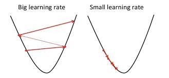
A small learning rate is more accurate at the cost of being more computationally expensive, on the other hand, a large learning rate is faster a the cost of the accuracy of the algorithm.
-
What are some drawbacks of Gradient descent?
Convergence to a local minimum might be extremely sluggish.
There is no guarantee that the algorithm will locate the global minimum if there are many local minima.
Key Takeaways
This article should provide you with a general understanding of the gradient descent method in machine learning. In this post, we looked at how a Gradient Descent method works, when it may be utilized, and what typical issues arise while utilizing it.
If you’re interested in learning more about Machine Learning, you should definitely check this course out!
Happy Learning!
