Do you think IIT Guwahati certified course can help you in your career?
Introduction
Let us get to the basics of training a neural network. While training a neural network, we make a forward propagation and calculate the cost of the neural network and later use the total calculated cost to backpropagate through the layers and update the weights; this process is done until the global minima is obtained. But this technique is efficient on small neural networks(neural networks with a small number of hidden layers).
In the case of large neural networks, traditional training methods are not efficient as it leads to vanishing gradient problem.
Vanishing gradient problem: All the layers using definite activation functions are added to neural networks. The gradients of the loss function tend to zero while backpropagating, making the network hard to train.
Due to this problem, the weights near the input layer will not be updated; only the weights near the output layer get updated.
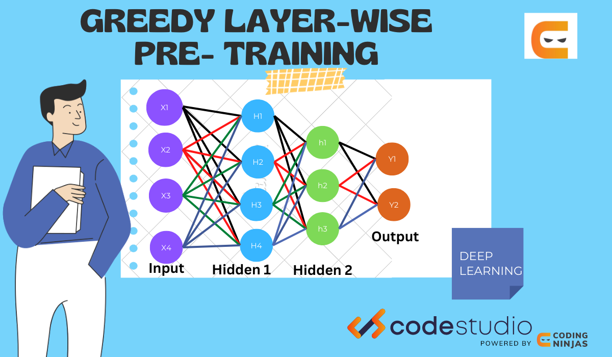
To solve the vanishing gradient descent problem, we use this technique. Lets us see the mechanism of a greedy layer-wise pretraining method. First, we make a base model of the input and output layer; later, we train the model using the available dataset. After training the model, we remove the output layer and store it in another variable. Add a new hidden layer in the model that will be the first hidden layer of the model and re-add the output layer in the model. Now there are three layers in the model, the input layer, the hidden layer1, and the output layer, and once again, train the model after inserting the hidden layer1. To add one more hidden layer, remove the output layer set all the layers as non-trainable(no further change in weights of the input layer and hidden layer1). Now insert the new hidden layer2 in the model and re-add the output layer. Train the model after inserting the new hidden layer. The model structure will be in the following order, input layer, hidden layer1, hidden layer2, output layer. Repeat the above steps for every new hidden layer you want to add. (each time you insert a new hidden layer, perform training on the model using the same dataset)
Multiclass Classification problem
To understand the greedy layer-wise pre-training, we will be making a classification model.
The dataset includes two input features and one output. The output will be classified into four categories. The two input features will represent the X and Y coordinate for two features, respectively. There will be a standard deviation of 2.0 for every point in the dataset. The random state will also be set to 2.
We will use the sklearn library for creating the dataset. The make_blobs() function is used to make the data points. Matplotlib is used to plot the dataset.
Creating and plotting dataset
Code for creating the dataset and plotting it.
# importing libraries and functions from matplotlib import pyplot as plt from numpy import where as wh from sklearn.datasets import make_blobs
# creating the 2-d dataset that is categorised into three parts x, y = make_blobs(n_samples=500, centers=4, n_features=2, cluster_std=2, random_state=2)
# scatter plot for each class value for i in range(4): # selecting indices of similar class labels row = wh(y == i) # plotting scatter points according to categories( different color for different category) plt.scatter(x[row, 0], x[row, 1]) # show plot plt.show()
Supervised Greedy Layer-Wise Pretraining
After creating the dataset, we will be preparing the deep multilayer perceptron(MLP) model. We will implement greedy layer-wise supervised learning for preparing the MLP model.
We do not require pretraining to address this simple predictive modeling problem. The main aim behind implementing the model is to perform a supervised greedy layer-wise pretraining model that can be used as a standard template and further used in larger datasets.
We will be using the dataset that was created earlier. To train a model using keras sequential, we must convert the output data to one-hot encoding. For that purpose, we will use the to_categorical() function from TensorFlow to convert the y into a one-hot encoding format.
from tensorflow.keras.utils import to_categorical
from tensorflow.keras.utils import to_categorical y = to_categorical(y)
The dataset has 500 points and splitting the dataset in the ratio of 9:1. 90% for training and the rest 10% for testing the model. Distributing the dataset into the training and testing part. For that, we will be using the train_test_split() function from the sklearn library.
from sklearn.model_selection import train_test_split xtrain, xtest, ytrain, ytest = train_test_split(x, y, test_size=0.1, random_state=42)
Next, we can train and create a base model.
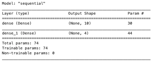
This will be a Multilayer Perceptron that expects two inputs for the two input variables in the dataset. It will have one hidden layer with 10 nodes and the Relu(rectified linear) activation function. The output layer has four nodes to predict the probability for each of the four classes and uses the softmax activation function.
# defining model model = Sequential() model.add( Dense(10, activation='relu', input_dim=2, kernel_initializer='he_uniform')) model.add( Dense(4, activation='softmax') )
We will compile the model using the Adam optimizer and the categorical_crossentropy loss function.
# compiling the model model.compile(loss='categorical_crossentropy', optimizer='Adam', metrics=['accuracy'])
Training the model in hundred epochs.
# fit model model.fit(xtrain, ytrain, epochs=100, verbose=0)
Printing the summary of the model.
Creating a function that will evaluate the model.
# evaluate a fit model defevaluate_model(model, xtrain, xtest, ytrain, ytest): _, train_acc = model.evaluate(xtrain, ytrain, verbose=0) _, test_acc = model.evaluate(xtest, ytest, verbose=0) return train_acc, test_acc
Evaluating the model.
# evaluate the base model scores = dict() train_acc, test_acc = evaluate_model(model, xtrain, xtest, ytrain, ytest) print('> Number of layers in model=%d, train=%.3f, test=%.3f' % (len(model.layers), train_acc, test_acc))
> Number of layers in model=2, train=0.789, test=0.860
We have prepared the base model of MLP now that we can outline the greedy layer-wise pretraining process.
For greedy layer-wise pretraining, we need to create a function that can add a new hidden layer in the model and can update weights in output and newly added hidden layers.
To make such a function, we need to store the output layer(last layer), including its configuration and weights. After storing the output layer, we will pop the output layer from the sequential model and now mark the layers as untrainable so that further update of these layers should not be possible. Add the new hidden layer and insert the output layer in the sequential model. Train the model after including the new hidden layer. Repeat this process for the number of layers you want to include in your MLP.
Function that adds a new hidden layer to the model.
# add one new layer and re-train only the new layer defadd_layer(model, xtrain, ytrain): # storing the output layer output_layer = model.layers[-1] # removing the output layer model.pop() # marking all the layers as un-trainable for layer in model.layers: layer.trainable = False # adding a new hidden layer model.add(Dense(10, activation='relu', kernel_initializer='he_uniform')) # adding the output layer model.add(output_layer) # fit model model.fit(xtrain, ytrain, epochs=100, verbose=0)
We are adding 10 new hidden layers.
# add layers and evaluate the updated model n_layers = 10 for i in range(n_layers): # adding a layer add_layer(model, xtrain, ytrain) # evaluating the model train_acc, test_acc = evaluate_model(model, xtrain, xtest, ytrain, ytest) print('> Number of layers in model=%d, train=%.3f, test=%.3f' % (len(model.layers), train_acc, test_acc)) # storing scores for plotting the graph scores[len(model.layers)] = (train_acc, test_acc)
Accuracy after adding each layer.
> Number of layers in model=3, train=0.844, test=0.860 > Number of layers in model=4, train=0.851, test=0.900 > Number of layers in model=5, train=0.847, test=0.900 > Number of layers in model=6, train=0.851, test=0.900 > Number of layers in model=7, train=0.856, test=0.900 > Number of layers in model=8, train=0.849, test=0.900 > Number of layers in model=9, train=0.858, test=0.900 > Number of layers in model=10, train=0.853, test=0.900 > Number of layers in model=11, train=0.853, test=0.900 > Number of layers in model=12, train=0.853, test=0.900
Plot the accuracy graphs after adding each layer.
# plot number of added layers vs accuracy plt.plot(list(scores.keys()), [scores[i][0] for i in scores.keys()], label='train', marker='*', color = 'red') plt.plot(list(scores.keys()), [scores[i][1] for i in scores.keys()], label='test', marker='*', color = 'blue') plt.legend() plt.show()
Layerwise learning is a method where individual components of a circuit are added to the training routine successively. Layer-wise learning is used to optimize deep multi-layered neural networks. In layer-wise learning, the first step is to initialize the weights of each layer one by one, except the output layer, and then train the data set.
What is greedy training?
Greedy layer-wise pretraining provides a way to develop deep multi-layered neural networks whilst only ever training shallow networks. Pretraining can iteratively deepen a supervised or unsupervised model that can be repurposed as a supervised model.
What is pre-training in deep learning?
Pre-training in AI refers to training a model with one task to help it form parameters that can be used in other tasks. Pre-training is a key method in studying and using deep convolutional neural networks. Greedy algorithm training is a technique used to pretrain deep belief networks.
What are the three layers of deep learning?
The neural networks in deep learning consist of the Input layer, Hidden layer, and Output layer. The hidden layer is also known as the processing layer. The input layer will accept the data, and the hidden layer will process it, giving neural networks exceptional performance. The outcome is stored in the output layer.
Which algorithm is used to train deep networks?
Deep learning models use several algorithms to train data sets. To extract features, classify objects, and identify relevant data patterns, algorithms use unknown elements in the input distribution throughout the training phase. The Greedy layer-wise pertaining is one of the methods used to train deep belief networks. It is used to develop deep multi-layered neural networks.
How many layers are there in a deep learning network?
A deep learning network has more than three layers (including input and output). There are four types of neural network layers in deep learning neural networks based on the type of network. These are Fully connected, Convolution, Deconvolution, and Recurrent network layers.
Conclusion
In this article, we have discussed the following topics:
Why use greedy layer-wise pretraining?
Mechanism of greedy layer-wise pretraining.
Implementation of greedy layer-wise pretraining model.


 9+ registered

