


Introduction
MS Excel gives us many features to manipulate our data and represent them in different forms; one of them is pivot tables. A pivot table is a table of grouped values that groups individual items from a more extensive table into one or more discrete categories.
We will learn about the grouping of pivot table items by having a pivot table in this blog.
Reading this blog will enhance your knowledge of MS Excel, and you will know everything about the grouping of pivot table items.
So, don't you want to get a clearer view of data by grouping your items in the pivot table? Let's directly move into the topic.
Group Pivot Table Items
We will see some examples to learn the grouping of pivot table items.
Here you will find one pivot table which we will use in examples-

Grouping of Products
In this pivot table, we want to make Group 1 of Apple, Banana, Cherry, and Group 2 of Orange, Pineapple, Watermelon. For creating these two groups, we will follow the below steps-
1. Select Apple, Banana, Cherry in the pivot table.

2. Now, right-click and click on the group button.

3. In the pivot table, select Orange, Pineapple, Watermelon.

4. Now, right-click and click on the group button.

Note- We can collapse and expand the groups by using the plus and minus buttons beside the group name.
Grouping of Dates
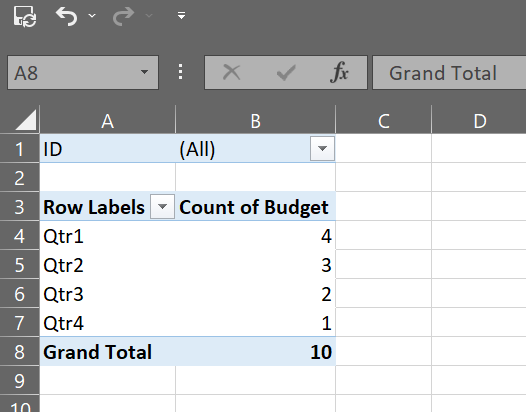
Instead of the Product field, add the Date of Purchase field to the Rows area to produce the pivot table below. There are a lot of entries in the Date of Purchase area: 6-January, 7-February, 22-January, 12-June, and so on.

Execute the procedures below to divide these dates into quarters.
1. Select any cell in the pivot table.
2. Now, right-click and click on the group button.
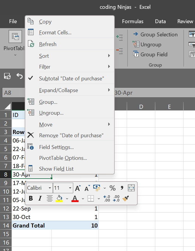
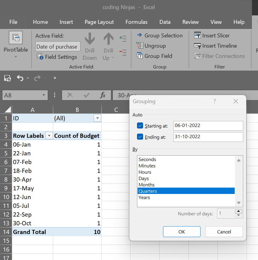
3. A dialogue box will appear, then select Quarters and click on the OK button.
Result-


 9+ registered

