Guided Backpropagation

Introduction

When it comes to extracting features from the images, convolutional networks play a great role in it. It performs various tasks like image classification, image captioning, object detection, image segmentation, visual question answering, etc. While these models provide higher performance, they are difficult to grasp due to their lack of decomposability into individually intuitive components. You might have often gone through a situation where you cannot figure out why the model is not showing satisfactory results for your use case, which leads you to various speculations about the code, adversarial attack, model architecture, hyper-parameters, Dataset, etc.

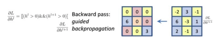
Guided Backpropagation is the combination of vanilla backpropagation at ReLUs and DeconvNets. ReLU is an activation function that deactivates the negative neurons. DeconvNets are simply the deconvolution and unpooling layers. We are only interested in knowing what image features the neuron detects. So when propagating the gradient, we set all the negative gradients to 0. We don’t care if a pixel “suppresses’’ (negative value) a neuron somewhere along the part to our neuron. Value in the filter map greater than zero signifies the pixel importance, which is overlapped with the input image to show which pixel from the input image contributed the most.

Working of Guided Backpropagation

RELU function during forward propagation.

^source

RELU function during backward propagation.

^source

Deconvolution for relu: The data having value greater than zero is flowing backward.

^source

Guided backpropagation combining both backward propagation and deconvolution.

^source

Implementation

Here is an implementation of a convolution neural network where we have used guided backward propagation that helps us to visualize fine-grained details in an image.

First, we will import all the necessary libraries that we are going to import to make a model.

#importing libraries
import numpy as np

import cv2
import tensorflow as tf
import matplotlib.pyplot as plt
%matplotlib inline
import tensorflow.keras.backend as K
from skimage.transform import resize

Now we will import an image and the last layer for VGG19 convolution network.

# setting the image path
image = 'img.jpg'
# setting the last conv layer for VGG19
Layer = 'block5_conv4'

Loading the image

img = tf.keras.preprocessing.image.load_img(image, target_size=(224, 224))

Displaying the original image.

plt.axis("off")
plt.imshow(img)
plt.show()

Let us preprocess the image by using the VGG19’s preprocess function.

# converts PIL image to numpy array
img = tf.keras.preprocessing.image.img_to_array(img)
# expanding the shape of the img array
x = np.expand_dims(img, axis=0)
# preprocess numpy array encoding to a batch of images
preprocessed_input = tf.keras.applications.vgg19.preprocess_input(x)

Importing the VGG19 transfered learning model on the imagenet dataset.

model = tf.keras.applications.vgg19.VGG19(weights='imagenet', include_top=True)

We are creating a model until the last convolution layer from the imported VGG19 transferred learning model. When we use the fully connected layer in the deep learning CNN model, we lose the spatial information which is retained by convolution layers.

gb_model = tf.keras.models.Model(
inputs = [model.inputs],
outputs = [model.get_layer(Layer).output]
)
layer_dict = [layer for layer in gb_model.layers[1:] if hasattr(layer,'activation')]

Gradients of ReLU are overridden by applying @tf.custom_gradient that allows the fine-grained control over the gradients for backpropagating non-negative gradients to have a more efficient or numerically stable gradient.

@tf.custom_gradient
def guidedRelu(a):
def grad(dy):
return tf.cast(dy>0,"float32") * tf.cast(a>0, "float32") * dy
return tf.nn.relu(a), grad

Applying the guided ReLU function to all the convolution layers wherever the activation function was ReLU.

for l in layer_d:
if l.activation == tf.keras.activations.relu:
l.activation = guidedRelu

We will use the Gradient tape to record the processed input image during the forward pass and calculate the gradients for the backward pass. Basically it is used to capture the gradients of the final(last) convolution layer.

with tf.GradientTape() as tp:
inputs = tf.cast(preprocessed_input, tf.float32)
tp.watch(inputs)
outputs = gb_model(inputs)[0]
grads = tp.gradient(outputs,inputs)[0]

Finally, visualizing the guided backpropagation.

#Visualizing the guided back prop
gb_prop = grads
guided_back_viz = np.dstack((
gb_prop[:, :, 0],
gb_prop[:, :, 1],
gb_prop[:, :, 2],
))
guided_back_viz -= np.min(guided_back_viz)
guided_back_viz /= guided_back_viz.max()

imgplot = plt.imshow(guided_back_viz)
plt.axis("off")
plt.show()

Here is an overall comparison of two images (input vs output).

Frequently Asked Questions

1. What is guided backpropagation?

A: Guided backpropagation visualizes fine-grained details in the image.

It says that neurons act like detectors for particular image features. While backpropagating the neurons with negative values are set to zero so that import pixels of the images get highlighted.

2. What is deconvolution?

A: Deconvolution refers to the operation that gets performed when the necessary computation is being done from the output layer to the input layer during error propagation or segmented image generation as in semantic segmentation.

3. What is the use of the ReLU activation function?

A: ReLU can be termed as rectified linear activation function. In short, a piecewise linear function will output the input zero if it is negative; otherwise, the output will be the same as the input. The graph of ReLU is shown below.

4. What is the use of guided backpropagation?

A: Guided backpropagation is used to capture pixels that are detected by the neurons, discarding the pixels that suppress the neurons. When backpropagating via ReLU layers, guided backpropagation calculates the gradient of the intended output with respect to the input, suppressing negative gradients.