Histogram Equalization in Digital Image Processing

What is Histogram Equalization?

Histogram Equalization is a specific intensity transformation technique used to enhance the contrast of an image. It works by spreading out the most frequent intensity values over a wider range, making low-contrast images look more detailed and clearer. This technique is especially useful in images where pixel intensity values are clustered within a narrow range, such as in medical or satellite imagery.

How Does Histogram Equalization Work?

1. Calculate the Histogram: First, you calculate the histogram of the image, which shows the distribution of pixel intensities.
    
2. Create a Cumulative Distribution Function (CDF): The CDF is then computed from the histogram, which helps to spread the pixel values.
    
3. Apply the Transformation: Finally, the pixel intensities of the image are mapped using the CDF to achieve a more balanced contrast.
    

Python implementation to perform histogram equalization using OpenCV:

• Python

Python

import cv2
import numpy as np
from matplotlib import pyplot as plt
import urllib.request

# URL of a chessboard image from the OpenCV GitHub repository
url = 'https://raw.githubusercontent.com/opencv/opencv/master/samples/data/left01.jpg'

# Download the image from the URL
resp = urllib.request.urlopen(url)
image_array = np.asarray(bytearray(resp.read()), dtype=np.uint8)

# Convert the image to grayscale
image = cv2.imdecode(image_array, cv2.IMREAD_GRAYSCALE)

# Apply Histogram Equalization
equalized_image = cv2.equalizeHist(image)

# Display the original and equalized images using matplotlib
plt.subplot(1, 2, 1)
plt.imshow(image, cmap='gray')
plt.title('Original Image')

plt.subplot(1, 2, 2)
plt.imshow(equalized_image, cmap='gray')
plt.title('Equalized Image')

plt.show()

You can also try this code with Online Python Compiler

Run Code

Output

Explanation

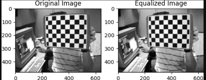
The output of the chessboard code will display two images side by side:

• Left Image: The original grayscale image of a chessboard.
   
• Right Image: The equalized image of the same chessboard, where the contrast has been enhanced using histogram equalization.
   

In the equalized image, you will observe a noticeable improvement in contrast. Darker areas will appear brighter, and brighter areas may appear slightly darker, making the overall image clearer. This is particularly helpful for highlighting details that may be hard to distinguish in the original image due to low contrast.

Time Complexity

• Calculating the histogram: The algorithm first needs to compute the histogram of pixel intensities, which takes O(N) time, where N is the total number of pixels in the image.
   
• Applying the transformation: Once the histogram is computed, the transformation function is applied to adjust the intensity levels across all pixels. This step also takes O(N) time.
   

Thus, the overall time complexity is O(N).

Space Complexity

The space complexity depends on:
 

• L, the number of intensity levels in the image, typically 256 for an 8-bit grayscale image.
   
• A small, constant amount of space is needed to store the histogram, which is an array of size L.

Thus, the space complexity is O(L), where L = 256 for grayscale images.

In summary:

• Time Complexity: O(N), where N is the number of pixels.
   
• Space Complexity: O(L), where L is the number of intensity levels (usually 256 for grayscale images).

Mathematical Derivation of Transformation Function for Histogram Equalization

The transformation function used in histogram equalization is derived using the cumulative distribution function (CDF). Let's break this down:

Calculate the Probability Distribution

Let n be the number of pixels in the image.

h(i) is the number of pixels with intensity i, so the probability of intensity i is:

p(i)= h(i)/n

Cumulative Distribution Function (CDF)

The CDF at intensity i is:

               i

CDF(i)= ∑​p(j)

              j=0

Transformation Function

The transformation function T(i) maps the original intensity to the new one, where L is the total number of intensity levels (usually 256 for grayscale images).

T(i)= round(CDF(i) X (L-1))

Steps Involved in Histogram Equalization

1. Compute Histogram: First, calculate the histogram of the image. A histogram is a graphical representation of the distribution of data points. In the context of an image, it represents the frequency of occurrence of each intensity level.
    
2. Calculate Cumulative Distribution Function (CDF): Transform the histogram into a cumulative histogram. This is essentially the cumulative distribution function (CDF) of the pixel intensities.
    
3. Normalize the CDF: The CDF must be normalized so that the range is between the minimum and maximum possible intensity values of the image. This scaling ensures that the output image has the appropriate brightness.
    
4. Create Equalized Histogram: Use the normalized CDF to map the intensity levels of the original image to new ones, which spreads the intensities more uniformly across the available range. This remapping is done by replacing each pixel in the input image with its corresponding value in the normalized CDF.
    
5. Generate Output Image: The final image is constructed using the new intensity values provided by the equalized histogram. This image will show enhanced contrast if the original image had a limited dynamic range.

Algorithm Overview

1. Compute the histogram (H) of the input image.
 

2. Compute the cumulative sum of the histogram to get the CDF: CDF(v) = sum(H(u) for u = 0 to v)
 

3. Normalize the CDF so that it ranges from 0 to the maximum pixel value: CDF_normalized = (CDF - CDF_min) * (Max_pixel_value / (Total_number_of_pixels - CDF_min))
 

4. Remap the pixel values of the original image using the normalized CDF to get the new pixel values.
 

5. Construct the output image using the new pixel values, resulting in enhanced contrast.
 

This process effectively redistributes the image's pixels in terms of intensity, leading to a generally better visualization of details and textures in the image due to the increased dynamic range. This technique is particularly useful in improving the quality of medical images, satellite images, and photographs taken in poor lighting conditions.

Example of Histogram Equalization in DIP

Let’s assume an image has only four intensity levels (0, 1, 2, 3) with pixel distribution as follows:

• 0: 40 pixels
   
• 1: 30 pixels
   
• 2: 20 pixels
   
• 3: 10 pixels

Calculate the Probability

p(0)=40/100​=0.4,p(1)=30/100=0.3,p(2)=20/100​=0.2,p(3)=10/100​=0.1

Calculate the CDF

CDF(0)=0.4,CDF(1)=0.4+0.3=0.7,CDF(2)=0.7+0.2=0.9,CDF(3)=0.9+0.1=1.0

Apply the Transformation

T(0)=round(0.4×3)=1,T(1)=round(0.7×3)=2,T(2)=round(0.9×3)=3,T(3)=round(1.0×3)=3

The new pixel values after histogram equalization would be 1, 2, 3, and 3.

Implementation

Let’s implement this example using Python to show how histogram equalization works on a small dataset:

• Python

Python

import numpy as np

import cv2

# Example pixel intensity values (4 levels)

image = np.array([[0, 0, 1], [1, 2, 2], [3, 3, 3]], dtype=np.uint8)

# Apply Histogram Equalization

equalized_image = cv2.equalizeHist(image)

# Print the equalized image

print("Equalized Image:\n", equalized_image)

You can also try this code with Online Python Compiler

Run Code

Output

Equalized Image:
 [[1 1 2]
 [2 3 3]
 [3 3 3]]

This demonstrates the pixel values after applying histogram equalization.

Benefits of Histogram Equalization

• Enhances the overall contrast of an image, especially in cases of poor lighting or low contrast.
• Improves the visibility of details in both bright and dark regions simultaneously.
• Simplifies image analysis tasks by creating a more uniform intensity distribution.
• Makes features more distinguishable for applications like medical imaging and remote sensing.
• Requires minimal computational resources and is easy to implement.
• Helps in preprocessing images for better performance in computer vision algorithms.

Limitations of Histogram Equalization

• May cause over-enhancement, leading to unrealistic or overly bright images.
• Does not preserve the natural appearance of images with already balanced contrast.
• Introduces noise or artifacts in areas with low-intensity gradients.
• Cannot handle images with highly localized brightness variations effectively.
• Produces non-optimal results when applied to color images without separating channels.
• Does not adapt well to images with distinct foreground and background intensities.

Frequently Asked Questions

Can histogram equalization enhance an overexposed or underexposed image?

Yes, histogram equalization can enhance underexposed or overexposed images by redistributing pixel intensities across the available range, improving contrast and revealing hidden details in dark or bright regions.

What are some real-world applications of histogram equalization?

Histogram equalization is used in medical imaging (e.g., X-rays), satellite image processing, object detection, facial recognition, and surveillance systems to enhance image clarity, improve feature visibility, and support better analysis and decision-making.

How does histogram equalization compare to other contrast enhancement techniques?

Histogram equalization provides global contrast enhancement, but it can over-enhance images. Other methods, like CLAHE (Contrast Limited Adaptive Histogram Equalization), offer localized adjustments, avoiding artifacts and maintaining natural appearance in regions with varying brightness.

Can histogram equalization be applied to color images? 

Yes, histogram equalization can be applied to color images by equalizing each channel (R, G, B) individually or by converting the image to grayscale.

Conclusion

In this article, we have explored Histogram Equalization in Image Processing which is key technique for enhancing image contrast. By redistributing pixel intensity values, it improves the interpretability of images in various fields.We discussed its mathematical foundation and provided a Python code implementation to demonstrate how the technique works. Understanding histogram equalization is essential for anyone interested in working with image processing, especially for enhancing images for visual and analytical purposes.

You can also check out our other blogs on Code360.