HLOOKUP Function

Introduction

The HLOOKUP function is used to find and retrieve a value from data in a horizontal table.

The “H” in the function name stands for horizontal. Thus this means Horizontal Lookup. The lookup values must appear in the first row of the table and move horizontally to the right.

Excel HLOOKUP Function

The purpose of this function is to look for a value in a table arranged horizontally.

The return value is the matched value from the table.

SYNTAX -

“=HLOOKUP (lookup_value, table_array, row_index, [range_lookup])”

ARGUMENTS -

lookup_value refers to the value that we want to look up.

table_array is the table from which we want to retrieve the value/data.

row_index is the row from which we want to retrieve the data.

range_lookup is optional. It is a boolean value that indicates an exact match or approximate match. (TRUE is the default value which refers to the approximate match)

EXAMPLES

Approximate Match

Source

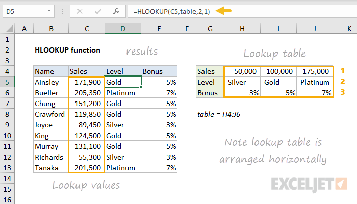
The sales amount is in C5:C13, and the lookup table is H4:J6. Our goal is to find the best match and not an exact match(for each value in C5:C13). To get the level and bonus, we need to change the row_index. The range_lookup will be set to 1, which will refer to the approximate match.

1. =HLOOKUP(C5, table, 2, 1)
   //this will get the level.
2. =HLOOKUP(C5, table, 3, 1)
   //this will get the bonus
    

Exact Match

Source

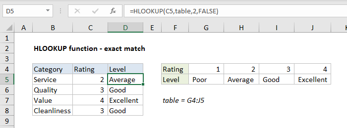
This is an example of an Exact match. Here we will be looking up the correct level for a numeric string 1-4. The table is G4:J5. The range_lookup will be set to FALSE for an exact match.

1. =HLOOKUP(C5, table, 2, FALSE)
   //exact match

Points to Note

1. When the range_lookup is set to False, it requires an exact match.
    
2. When the range_lookup is omitted or True, and no exact match is found, the function will look for the nearest value in the table(less than the lookup value).
    
3. When range_lookup is True, the lookup values of the first row of the table must be sorted in ascending order; else, it may return an incorrect answer. But when it is an Exact match situation, the values need not be sorted.