Do you think IIT Guwahati certified course can help you in your career?
Introduction
An image is a picture that is formed by actual existence. The image is the main means for people to obtain information from the outside world—the key work of image recognition.
This process involves delving into the representation of input images, allowing the machine to enhance its comprehension independently. The objective is to enable the machine to recognize and classify these images autonomously. The procedure encompasses external input samples subjected to various devices and filters, isolating pivotal features within the input images.
This comprehensive approach ultimately facilitates the accomplishment of image recognition and classification tasks. Image recognition involves a wide range of research content, such as license plate recognition, handwritten digit recognition, face recognition, and recognition and classification of parts in machining and accurate weather forecasting based on meteorological satellite photos.
In this article, we learn about implementing Deep Autoencoder in PyTorch.
What is PyTorch?
It is a schematic diagram of Dropout. When training the Dropout method, the output value is calculated by the activation function of the hidden layer node. It is randomly cleared during the forward transmission. Pytorch is the input connected to the hidden layer neurons.
The weights are randomly removed with a certain probability. It is a schematic diagram of a Pytorch. In other words, the fully connected six layers become sparsely connected. Using the Pytorch method, its connections are randomly selected during the training phase.
It should be noted that this does not mean that the weight matrix. It is set to a fixed sparse matrix. During the training process because, during each training. The weights are randomly cleared and not settled each time.
Deep Autoencoder
Autoencoders usually use a stacked structure in practical applications. Applying stacked autoencoders eliminates the huge workload of manually extracting data features. It improves the efficiency of feature extraction. It also exhibits powerful learning capabilities.
Our model employs a 2-layer AE. The idea of Pytorch is introduced in the first layer of AE. Pytorch is a new regularization method proposed by Wan et al.
After introducing the Pytorch idea, the input and hidden layers are no longer connected. But they are randomly connected so that the dynamic sparseness of the network can be achieved.
Implement Deep Autoencoder in PyTorch
Step 1: Setting Up the Environment
Install the required packages using the following command. Make sure you have Python and PyTorch installed on your system.
pip install torch numpy matplotlib
Step 2: Dataset Selection and Preprocessing
We'll make use of the torch-vision library to load the dataset.
import torch
from torchvision import datasets
from torchvision import transforms
import matplotlib.pyplot as plt
import torch.nn as nn
import torchvision
import torchvision.transforms as transforms
import matplotlib.pyplot as plt
We are using PyTorch's nn. Module class, we'll build an encoder and a decoder. Our deep autoencoder's encoder and decoder parts will each have several fully connected layers. The architecture can be defined as follows:
We use the Mean Squared Error loss function to determine how much the input and reconstructed data differ. We'll train our model using the Adam optimizer:
model = Autoenc()
loss_function = torch.nn.MSELoss()
optimizer = torch.optim.Adam(model.parameters(), lr = 1e-1, weight_decay = 1e8)
Step 5: Training the Model
Assessing how well our deep autoencoder has learned to reconstruct the input data after training is critical. To evaluate the accuracy of the reconstruction, we can compare the original and reconstructed images:
# Hyperparameters
epochs = 10
batch_size = 128
learning_rate = 0.001


# Lists to store losses and outputs
losses = []
outputs = []

# Training loop
for epoch in range(epochs):
    for (image, _) in loader:
        image = image.view(-1, 28 * 28)

        reconstructed = model(image)

        loss = loss_function(reconstructed, image)

        optimizer.zero_grad()
        loss.backward()
        optimizer.step()

        losses.append(loss.item())  # Append loss value to the list

    outputs.append((epoch, image, reconstructed))
Step 6: Evaluating Model Performance
Beyond image reconstruction, autoencoders can be used for a variety of purposes.
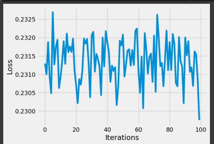
# Plotting the loss
plt.style.use('fivethirtyeight')
plt.xlabel('Iterations')
plt.ylabel('Loss')
plt.plot(losses[-100:])
plt.show()
# ...
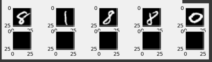
# Displaying original and reconstructed images
with torch.no_grad():
for epoch, image, reconstructed in outputs:
plt.figure(figsize=(9, 2))
for i in range(5):
plt.subplot(2, 5, i + 1)
plt.imshow(image[i].view(28, 28).detach().numpy(), cmap='gray')
plt.subplot(2, 5, i + 6)
plt.imshow(reconstructed[i].view(28, 28).detach().numpy(), cmap='gray')
plt.show()
break
Output
Frequently Asked Questions
What is the Boltzmann Machine?
A network of symmetrically connected, neuronlike units that make stochastic decisions. Boltzmann machines have a learning algorithm that allows them to discover interesting features in datasets composed of binary vectors.
What is the Sigmoid Function?
A sigmoid function also called a logistic function, is an “S”-shaped continuous function with domain over all R. However, the range is only over (0, 1).
What is Swish?
Swish is unbounded above and bounded below. Unlike ReLU, Swish is smooth and nonmonotonic. The non-monotonicity property of Swish distinguishes itself from the most common activation functions.
Conclusion
In this article, we learn about implementing Deep Autoencoder in PyTorch. We also learn about Deep Autoencoder and also PyTorch. We concluded the article by discussing the definition and implementation.


 9+ registered

