Implementation of Random Forest with Python

Implementation of Random Forest

We will now look up the Implementation of Random Forests. I have downloaded the Breast Cancer dataset from the Kaggle website. I will train my machine learning model using a random forest classifier to check the accuracy of the prediction. All I do is data cleaning and data manipulation. I have loaded the sample datasets in Google collab, and let's begin with data cleaning. 

First, import the libraries that we need during the program.

 

import pandas as pd
import numpy as np
import matplotlib.pyplot as plt
import seaborn as sns

 

Now read the CSV file that contains breast-cancer datasets.

 

df = pd.read_csv("breast-cancer.csv")

 

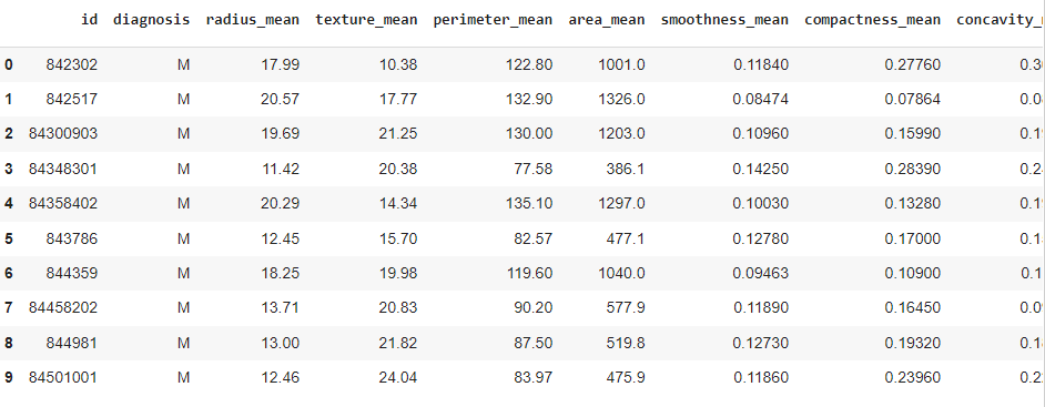
Once the dataset is in the data frame 'df,' let's print the first ten rows of the dataset. 

 

df.head(10)

Output:

 

 

There are various features (columns) in the dataset; let's check them out.

 

df.shape

 

Output:

 

 

So, there are 569 rows and 33 columns in the dataset. Let’s count the number of empty (Nan, NAN, na) values in each column.

 

df.isna().sum()

 

The above function gives the sum of all NaN values present in each of the features.

 

Output:

 

 

Column ‘Unnamed’ has 569 NaN values. So, we need to drop that column from the datasets.

Also, column ‘id’ doesn’t have any impact on predicting the output. So, we’ll drop this too.

 

df.drop(['Unnamed: 32','id'],axis='columns',inplace=True)

 

Now, let’s get the count of the number of Malignant(M) and Benign(B) cells in the diagnosis column.

 

df['diagnosis'].value_counts()

 

Output:

 

 

So, there are 357 Benign and 212 Malignant entries in the column ‘diagnosis’.

Let’s visualize the count of column ‘diagnosis’ using the seaborn library.

 

sns.countplot(df['diagnosis'])

 

Output:

 

It seems that Benign cases are more dominating than Malignant.

Now, I will encode the categorical values, i.e., Malignant(M) and Benign(B), with the help of a SKlearn library called LabelEncoder.

 

from sklearn.preprocessing import LabelEncoder

 

M is represented by the value 1, and B is represented by the value 0.

 

 

We explored the data, manipulated it, and cleaned it. It’s time to create a model to detect Cancer cells.

Split the datasets into Independent (X) and Dependent (Y) datasets.

 

X = df.iloc[:,1:31].values
Y = df.iloc[:,0].values

 

The Target or dependent variable is the diagnosis, and the Independent variables are all the features except 'diagnosis.' X and Y are NumPy arrays.

Now, split the datasets into 80% training and 20% testing. 

 

from sklearn.model_selection import train_test_split
X_train, X_test, Y_train, Y_test = train_test_split(X, Y, test_size = 0.2, random_state = 0)

Let’s scale the data to bring out the features to the same level. This means that the data would be within a specific range. This technique is called Feature Scaling.

from sklearn.preprocessing import StandardScaler
sc = StandardScaler()
X_train = sc.fit_transform(X_train)
X_test = sc.fit_transform(X_test)

 

Now, I will create a Decision Tree model to train the dataset. Let’s create a function for this.

 

def models(X_train, Y_train):
  #Random Forests Classifier
  from sklearn.ensemble import RandomForestClassifier
  forest = RandomForestClassifier(n_estimators = 10, criterion =  'entropy',  random_state = 0)
  forest.fit(X_train, Y_train)
  return forest

 

The above function trains the Model using X_train and Y_train datasets. Now, I will predict the Model's output on testing samples, i.e., X_test, and compare the score with Y_test.

 

model = models(X_train, Y_train)
model.score(X_test, Y_test)

 

 

The Model is doing very well. 97% of predictions are correct.

Let’s have a look at the predicted value of X_test by the Model.

 

pred = model[2].predict(X_test)

 

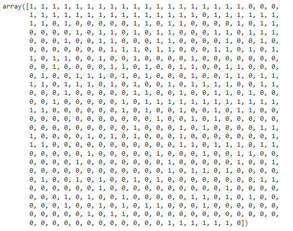
The actual value, i.e., Y_test, is:

 

 

 

 

Frequently Asked Questions

1. The Random Forest is good over Decision Tree because -
   => We prefer Random Forest over decision tree because there occurs Overfitting in Decision Tree.
    
2. Pick the correct option/s regarding using Decision Trees for regression-
   a) Predicted value is the mean of all the samples that belong to that node.
   b) Predicted value is the minimum of all the samples that belong to that node.
   c) Split is based on the accuracy
   d) Split is based on the MSE ( Mean Squared Error)
   
   -> a) Predicted value is the mean of all the samples that belong to that node.
        d) Split is based on the MSE ( Mean Squared Error)
    
3. What is Out-of-Bag Error?
   =>In the Random forest algorithm, there is no need for separate testing data to validate the result. As the forest is built on training data, each tree is tested on one-third of the samples not used in making that tree. This is known as the out-of-bag error, an internal error estimate of a Random forest as it is being constructed.
    
4. What are Bagging trees?
   => Bagging is the method to improve the performance by bundling the result of weak learners. In Bagging trees, individual trees are independent of each other.
    
5. What are Gradient boosting trees?
   => In Gradient boosting trees, we introduce a new regression tree to compensate for the shortcomings of the existing model. We can use the Gradient Descent algorithm to minimize the loss function.

 

Key Takeaways

In this blog, I discussed the brief Introduction and Implementation of Decision Trees from Scratch. For more information, you must visit here.

( must check: NAIVE BAYES IMPLEMENTATION )

 

Thank You 😊😊