Implementing Linear Models Using scikit-learn

Introduction

Hello, Ninjas! Welcome again. Before jumping to an article, I would like to ask you a question Have you ever wondered how you can forecast sales? Resource consumption? Telecom services lifestyle forecasting?

Let me tell you all you can do with implementing linear models using scikit-learn.

In this article, we’ll see a basic introduction to linear models in machine learning. We’ll mathematically explore the two types of regularisation and see the implementation of these techniques to overcome the issue of overfitting in a model.

Linear Regression

Linear Regression is a linear model, i.e., a model which is used to predict the value of a variable (dependent variable ‘Y’) based on the value of another variable (Independent variable ‘X’)

• Dependent Variable(Y) – The variable whose value you want to predict.
   
• Independent Variable(X) – The variable you use to predict the other variable’s value is called the independent variable.
   

There are two types of linear regression based on the no. of dependent variables (also called input variables). 

Simple Linear Regression when there is a single dependent variable & Multiple Linear Regression when there are multiple dependent variables.

To learn more about Linear Regression, follow this article,  

Prerequisite

For implementing a linear regression model using scikit-learn, you need to have basic knowledge of Machine Learning, and there are certain assumptions to implement the model they are all the variables are continuous and numeric, not categorical, and Data should be free of missing values and outliers, and there must be a linear relationship between predictor and predictions.

Ridge and Lasso Regression using Scikit-learn

Robust techniques like Ridge and Lasso regression are typically utilized to build efficient models when there are a large number of features. These regressions help simplify models and avoid over-fitting.

Ridge regression is the regularisation method that carries out L2 regularisation, i.e., adding a penalty equal to the square of the coefficients' magnitude. In contrast, Lasso regression is the regularisation method that carries out L1 regularisation, i.e., adds a penalty equal to the absolute value of the coefficients' magnitude.

Ridge Regression

As mentioned before, Ridge regression does "L2 regularisation," which is to say it increases the optimization objective by a sum of squares of the coefficients factor. Ridge regression, therefore, enhances the following:

Objective = RSS + α* (sum of the square of coefficients).

Here, the parameter α (alpha) balances the relative importance of minimizing the RSS and minimizing the sum of the squares of the coefficients. α has a range of possible values:

α = 0:

The objective is the same as it was with simple linear regression.

α = ∞:

Due to the infinite scaling factor on the square of the coefficients, the coefficients will be zero; otherwise, the objective will be unlimited.

0< α< ∞:

The weight assigned to various objective components will depend on the magnitude of α.

The coefficients for a simple linear regression will fall between 0 and 1.

Let’s see how to implement Ridge regression.

Import libraries such as NumPy, Pandas, and Matplotlib.pyplot

import numpy as np
import pandas as pd
import matplotlib.pyplot as plt

You can also try this code with Online Python Compiler

Run Code

Import the Data Set

from sklearn.datasets import load_diabetes
data=load_diabetes()
  print(data.DESCR)
x=data.data
y=data.target

from sklearn.model_selection import train_test_split
  x_train, x_test, y_train, y_test = train_test_split(x,y,test_size=0.2,random_state=45)

from sklearn.linear_model import LinearRegression
L=linearRegression()

  L.fit(x_train,y_train)

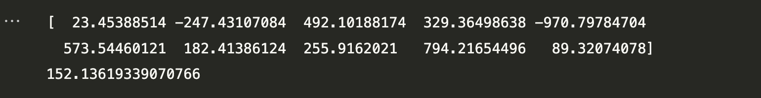
  print(L.coef_)
  print(L.intercept_)

You can also try this code with Online Python Compiler

Run Code

Output

from sklearn.linear_model import Ridge
  R=Ridge(alpha=100000)
  R.fit(x_train,y_train)

You can also try this code with Online Python Compiler

Run Code

Output

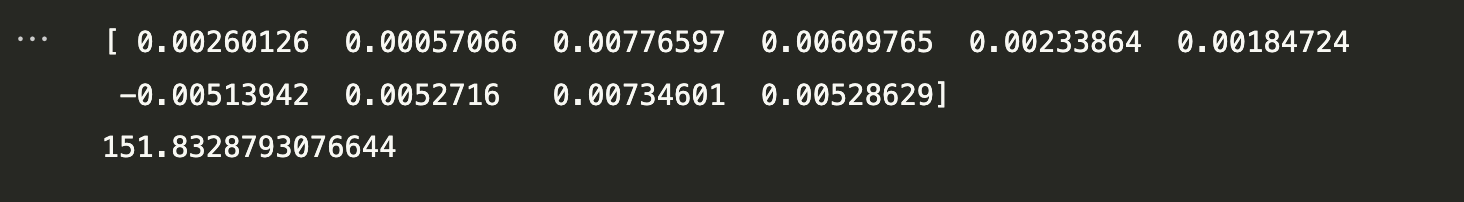
print(R.coef_)
print(R.intercept_)

You can also try this code with Online Python Compiler

Run Code

Output

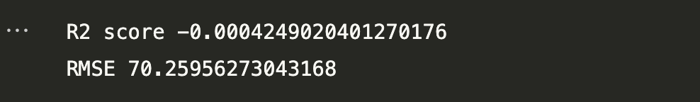
print("R2 score",r2_score(y_test,y_pred))
print("RMSE",np.sqrt(mean_squared_error(y_test,y_pred)))

You can also try this code with Online Python Compiler

Run Code

Output

Lasso Regression

Lasso regression implements L1 regularisation, which means adding a factor equal to the sum of absolute values of the coefficients in the optimization objective. As a result, lasso regression enhances the following:

Objective: RSS + α * (sum of the absolute value of coefficients)

 
In this case, α (alpha) functions similarly to ridge and provides an exchange between regulating RSS and coefficient magnitude. Like ridge, can have a variety of values. Let us iterate briefly here:

• α= 0
  Coefficients are the same as in simple linear regression.
   
• α=∞
  All coefficients are zero (same logic as before).
   
• 0<α<∞ 
  Coefficients between 0 and the basic linear regression coefficients.
   

from sklearn.datasets import load_diabetes
 
import numpy as np
import pandas as pd
import matplotlib.pyplot as plt
 
from sklearn.linear_model import Lasso
from sklearn.metrics import r2_score
from sklearn.model_selection import train_test_split

You can also try this code with Online Python Compiler

Run Code

data = load_diabetes
df = pd.dataframe(data.data,columns=data.feature_names)
df['TARGET'] = data.target
df.head()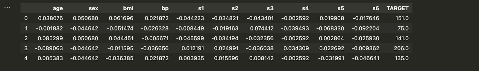

You can also try this code with Online Python Compiler

Run Code

Impact on Bias and Variance

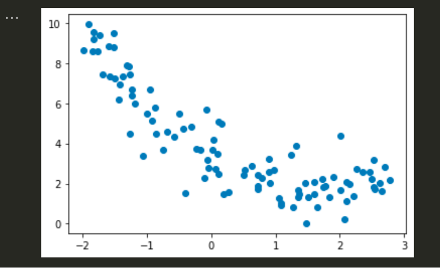
m = 100
X = 5 * np.random.rand(m, 1) - 2
y = 0.7 * X ** 2 - 2 * X + 3 + np.random.randn(m, 1)
 
plt.scatter(X, y)

You can also try this code with Online Python Compiler

Run Code

Output

X_train,X_test,y_train,y_test = train_test_split(X.reshape(100,1),y.reshape(100),test_size=0.2,random_state=2)

You can also try this code with Online Python Compiler

Run Code

from sklearn.preprocessing import PolynomialFeatures
poly = PolynomialFeatures(degree=10)
 
X_train = poly.fit_transform(X_train)
X_test = poly.transform(X_test)

You can also try this code with Online Python Compiler

Run Code

from mlxtend.evaluate import bias_variance_decomp
alphas = np.linspace(0,30,100)
loss = []
bias = []
variance = []
for i in alphas:
reg = Lasso(alpha=i)
avg_expected_loss, avg_bias, avg_var = bias_variance_decomp(
     reg, X_train, y_train, X_test, y_test,
     loss='mse',
     random_seed=123)
loss.append(avg_expected_loss)
bias.append(avg_bias)
variance.append(avg_var)
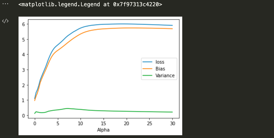
plt.plot(alphas,loss,label='loss')
plt.plot(alphas,bias,label='Bias')
plt.plot(alphas,variance,label='Variance')
plt.xlabel('Alpha')
plt.legend()

You can also try this code with Online Python Compiler

Run Code

Output

The effect on the bias and variance would look like

Effect of Regularization on Loss Function

from sklearn.datasets import make_regression
 
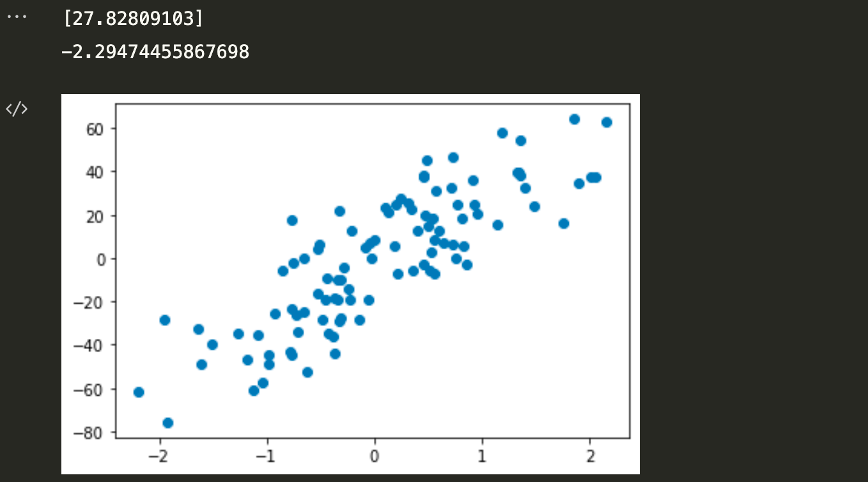
X,y = make_regression(n_samples=100, n_features=1, n_informative=1, n_targets=1,noise=20,random_state=13)
 
  plt.scatter(X,y)
 
from sklearn.linear_model import LinearRegression
 
  reg = LinearRegression()
    reg. fit(X,y)
  print(reg. coef_)
    print(reg. intercept_)

You can also try this code with Online Python Compiler

Run Code

Output

This is how the effect of regularization on the loss function.