Implementing Support Vector Machine

Step II

 

Exploratory Data Analysis on Breast Cancer Dataset.

Importing the dataset

 

# I have downloaded and saved the dataset in sample_data folder in Google Colab

data = pd.read_csv('./sample_data/Breast_cancer_data.csv')
data.head()

 

 

Shape, size, and measures of central tendency analysis

 

data.info()

 

data.describe()

 

 

Infographics of the relation between features

 

sns.pairplot(data, hue='diagnosis', vars=['mean_radius', 'mean_texture', 'mean_perimeter', 'mean_area', 'mean_smoothness']);

 

 

# Plotting the correlation matrix

plt.figure(figsize=(15, 12))
sns.heatmap(data.corr(), annot=True, cmap='Blues');

 

 

Missing values analysis

 

data.isna().sum()

 

Checking the dataset is balanced or not by plotting target values.

 

graph = sns.countplot(x='diagnosis', data=data);
for p in graph.patches:
  graph.annotate('{:.1f}'.format(p.get_height()), (p.get_x()+0.25, p.get_height()+0.01))

 

 

Step III

Making the dataset suitable for model training.

 

Splitting the dataset into training and testing - We’ll use the training dataset to train our SVM model for the predictions and the testing dataset to check the accuracy of the predictions.

 

# x contains all the independent features
# y is the target variable

x = data.drop(['diagnosis'], axis=1).values
y = data['diagnosis'].values

#splitting in training and testing
from sklearn.model_selection import train_test_split
x_train, x_test, y_train, y_test = train_test_split(x, y, test_size=0.25, random_state=101)

print("The training data has", x_train.shape[0], "records.")
print("The testing data has", x_test.shape[0], "records.")

 

 

Step IV

Training SVM Model

 

Importing the model and training the model on training dataset

 

from sklearn.svm import SVC
svc_model = SVC()

svc_model.fit(x_train, y_train)

 

Generating predictions

 

y_predict = svc_model.predict(x_test)
print(y_predict)

 

 

Step V

Evaluating our model

 

Printing classification reports and confusion matrix

 

from sklearn.metrics import classification_report, confusion_matrix

# Confusion Matrix
cm = confusion_matrix(y_test, y_predict)
sns.heatmap(cm, annot=True);

 

 

# Classification Report

cr = classification_report(y_test, y_predict)
print(cr)

 

 

Step VI

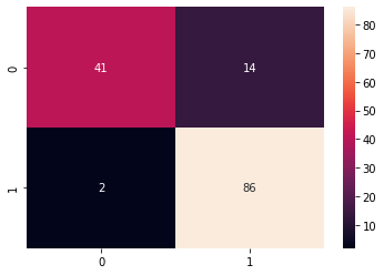
Results: The accuracy of our SVM model is 0.89, which is pretty good.

 

From the Confusion matrix, we can see the value of True Positives is 41, which means that 41 females have been correctly classified as ‘not having cancer’ and True Negatives is 86, which means that 86 females have correctly been classified as ‘having cancer.’

 

Our model has predicted that 55 (41 + 14) females don’t have breast cancer; hence the value of False Negative is 14.

 

The model also classified two females as ‘having cancer,’ but they didn’t have cancer in reality, so False Positive’s value is 2.

 

Frequently Asked Questions

 

1). What are the applications of SVMs?
Support Vector Machine has many use-cases in real-world projects like:

1. Face Detection,
2. Gene Classification,
3. Email Classification,
4. Handwriting Recognition

 

 

2). What is the use-case of SVM?

SVM is a supervised machine learning algorithm that can be used for classification or regression problems.

 

3). What is the standard Kernel Function equation?

The standard kernel function equation is:

Key Takeaways

 

Congratulations on making it this far. In this blog, we implemented a Support Vector Machine Algorithm using a Breast Cancer Dataset. Click here, If you want to learn the theoretical aspects of SVM. The kernel is essentially a function to perform calculations even in the higher dimensions in SVM. Learn more about Kernels from this blog.

You can also consider our Online Coding Courses such as the Machine Learning Course to give your career an edge over others.

If you are preparing for the upcoming Campus Placements, then don’t worry. Coding Ninjas has your back. Visit this link for a carefully crafted and designed course on-campus placements and interview preparation.