Table of contents
1.
Introduction
2.
Jointly Gaussian Random Variables
2.1.
Gaussian Random Variable 
2.2.
Jointly Gaussian Random Variable
2.2.1.
Probability Density Function for Jointly Gaussian Random Variable
2.3.
Covariance Matrix 
3.
Implementation of the Jointly Gaussian Random Variable
4.
Frequently Asked Questions
5.
Conclusion
Last Updated: Mar 27, 2024
Easy

Jointly Gaussian Random Variables

Author Tushar Tangri
0 upvote
Career growth poll
Do you think IIT Guwahati certified course can help you in your career?

Introduction

A bivariate normal distribution is formed by two independent random variables instead of the "ordinary" normal distribution, which includes just one random variable. The two variables are both normally distributed, and when they are put together, they have a normal distribution. A three-dimensional bell curve represents the jointly normal distribution visually.

In this blog, we will be discussing the most commonly used definition to define jointly gaussian random variables and start from its basics because the Gaussian distribution can be defined in a variety of ways; there is no universal agreement on a concise description. 

Jointly Gaussian Random Variables

Gaussian Random Variable 

In Gaussian Random variable, a random variable that is continuous and has a probability density function of the type 

Where µ is mean, and σ 2 is the variance.

N (µ, σ2 ) refers to a Gaussian distribution with mean µ and variance σ 2 

X ∼ N (µ, σ2 ) ⇒ X is a Random Gaussian variable with mean µ and variance σ 

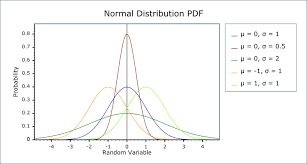
If X ∼ N (0, 1), X is a standard Gaussian Random variable.

The below diagram represents the figure for a standard gaussian random variable.   

Jointly Gaussian Random Variable

Let X1 and X2 be two variables. . . , and Xd is real-valued random variables that are established along with the same sample space.  If their joint characteristic function is provided by the equation below, they are said to be jointly Gaussian.


                                                                       Here p is the correlation of x1 and x2.

Gaussian random variables that are independently Gaussian are always jointly Gaussian. Below is a diagram of the two-dimensional joint Gaussian probability density function to understand this better. 

Source: Link

To compute its density, it is necessary to know the mean and variance of a linear combination of jointly Gaussian random variables.

Probability Density Function for Jointly Gaussian Random Variable

The two parameters, various discuss µ, and σ2, the first and second-order moments, are obtained from the pdf and are entirely defined by the Gaussian pdf P(x1) and P(x2). 

Source: Link

In the new basis, the joint Gaussian probability density function is a joint distribution given by  

This equation is used to present that each marginal probability density function in the new basis is an independent gaussian PDF, with each distribution having varied variance. 

Covariance Matrix 

A covariance matrix is a symmetrical matrix that can be diagnosed by changing the basis. Any joint Gaussian random variable pdf has a basis for which the pdf expressed is product distribution.  

A covariance Matrix is shown as follows in the below-given diagram:

Where the diagonal elements of Σ are referred to as the variance of random variables X and the generic elements Σij = E(Xi − mXi )(Xj − mXj ) is the covariance of the jointly gaussian random variables.  

A (symmetric) positive semi-definite matrix must be used as the covariance matrix cov. Because cov's determinants and inversion are computed as pseudo-determinant and pseudo-inverse, respectively, cov does not require complete rank.

The covariance matrix is the identity times that value if the parametric cov is a scalar, a vector of diagonal records for the covariance matrix if the parameter cov is a vector of diagonal records for the covariance matrix, or a two-dimensional array-like if the parameter cov is a two-dimensional array-like.

Implementation of the Jointly Gaussian Random Variable

Step 1: Import all the required libraries such as numpy, matplotlib, etc. 

import numpy as np
import matplotlib.pyplot as plt
from matplotlib import cm
from mpl_toolkits.mplot3d import Axes3D
You can also try this code with Online Python Compiler
Run Code


Step 2: Create a 2-dimensional distribution over variables X and Y. We take our N as 1000 to visualize over it. 

N = 1000
X = np.linspace(-3, 3, N)
Y = np.linspace(-3, 4, N)
X, Y = np.meshgrid(X, Y)
You can also try this code with Online Python Compiler
Run Code


Step 3: We create our mean vector and covariance matrix. We use mu for mean vectors and sigma to represent covariance matrix. 

mu = np.array([0, 1])
Sigma = np.array([[1 , 0.6], [0.6,  2]])
You can also try this code with Online Python Compiler
Run Code


Step 4: We pack X and Y into a single three-dimensional array to visualize our created data.

pos = np.empty(X.shape + (2,))
pos[:, :, 0] = X
pos[:, :, 1] = Y
You can also try this code with Online Python Compiler
Run Code


Step 5: Return the multivariate Gaussian distribution on array pos.

pos is an array constructed by packing the meshed arrays of variables

x_1, x_2, x_3, ..., x_k into its _last_ dimension.

def multivariate_gaussian(pos, mu, Sigma):

    n = mu.shape[0]
    Sigma_det = np.linalg.det(Sigma)
    Sigma_inv = np.linalg.inv(Sigma)
    N = np.sqrt((2*np.pi)**n * Sigma_det)
    # This einsum call calculates (x-mu)T.Sigma-1.(x-mu) in a vectorized

    # way across all the input variables.
    fac = np.einsum('...k,kl,...l->...', pos-mu, Sigma_inv, pos-mu)

    return np.exp(-fac / 2) / N
You can also try this code with Online Python Compiler
Run Code


Step 6: We assign the variable Z to mu, sigma, and pos values. 

Z = multivariate_gaussian(pos, mu, Sigma)
You can also try this code with Online Python Compiler
Run Code


Step 7: We create a surface plot and project a filled contour plot under it. 

ig = plt.figure()
ax = Axes3D(fig)
ax.plot_surface(X, Y, Z, rstride=3, cstride=3, linewidth=1, antialiased=False,
                cmap=cm.viridis)

cset = ax.contourf(X, Y, Z, zdir='z', offset=-0.15, cmap=cm.viridis)
You can also try this code with Online Python Compiler
Run Code


Step 8: In the last step, we need to adjust the limits, ticks, and view angle. 

ax.set_zlim(-0.15,0.2)
ax.set_zticks(np.linspace(0,0.2,5))
ax.view_init(27, -21)
ax.set_xlabel('X')
ax.set_ylabel('Y')
ax.set_zlabel('P D F', labelpad=1)
plt.title('Bivariate Normal Distribution (1000 samples)')
plt.savefig('1000bivariatePDF.png', dpi = 300)
plt.show()

iks = np.array([1,2])
fx = (1/(Sigma * np.sqrt(2 * np.pi)) *
            np.exp( - (iks - mu)**2 / (2 * Sigma**2) ))
print(iks, fx)
You can also try this code with Online Python Compiler
Run Code


Output:

Thus we have successfully visualized the implementation of the jointly Gaussian random variable in python for a better understanding of the concepts. 

Frequently Asked Questions

  1. How do we acknowledge that the given two variables are jointly Gaussian random variables?
    To confirm the fact that the two given variables are jointly Gaussian random variables, If aX+bY has a normal distribution for every a,b∈R, then the two random variables X and Y are said to be jointly gaussian random variables.
     
  2. How do we simulate the jointly gaussian random variable? 
    The conditional distribution of a random variable X2 given X1. As a result, a bivariate normal distribution may be simulated by selecting one random variable from the marginal normal distribution and another from the conditional normal distribution. 
     
  3. What is a jointly Gaussian random variable in python? 
    One or both variables might be discontinuous in the bivariate distribution histogram. Another technique to compare conditional univariate distributions is to plot one discrete and one continuous variable.  

Conclusion

In machine learning and data science, Gaussians are a required distribution. Knowing how to use them in multivariate circumstances in order to become a better data scientist or machine learning professional.  This article has thoroughly discussed the joint Gaussian random variable and all the required prerequisites such as joint Gaussian pdf, covariance matrix, and Gaussian random variable. We have also visualized how the jointly gaussian random variable works in practical-based scenarios.  
To learn more about similar concepts, follow our blogs to understand deep in machine learning. 
Check out this problem - Largest Rectangle in Histogram

Live masterclass