K-Nearest-Neighbor: Theory and Implementation

When should the KNN Algorithm be used?

If you have a small dataset with noise-free and labeled data, the KNN method is a good choice. When the data set is small, the classifier executes in a shorter amount of time. If your dataset is large, KNN is useless without any tweaks.

Advantage and Disadvantage of Using KNN

Advantages 

• Despite its simplicity, it produces incredibly competitive results. The usage of KNN in collaborative filtering algorithms for recommender systems is an excellent example of this. This algorithm is the method used behind Amazon's Recommender Systems' screens.
• It's a multi-purpose supervised machine learning algorithm that can solve regression, classification, and search issues.
• When designing a KNN model, there are three distance criteria to choose from: Euclidean, Manhattan, and Hamming distance. Depending on the type of dataset, each of the distance functions serves a particular purpose. It is possible to select the optimal solution based on the type of the features - Manhattan and Euclidean for numeric attributes and Hamming for categorical characteristics.

Disadvantages

• As the dataset grows, the algorithm's efficiency decreases rapidly.
• It has skewed class distributions, which means that if a particular class appears frequently in the training set, it is likely to dominate the majority voting of the new sample.
• It can't handle missing data, and to compute the distance, you’ll need a complete features vector for each instance. You can solve this problem by filling in the missing values with the feature's average value throughout the whole dataset.

Implementation

Here we will use the Glass Identification Data Set from UCI. To get more information on this dataset, refer to this link (Data Source). 

Our primary goal is to use the K Nearest Neighbor Classifier to classify data points based on their glass type.

Importing the required library

import numpy as np
import matplotlib.pyplot as plt
 
import pandas as pd  
import seaborn as sns
 
%matplotlib inline

You can also try this code with Online Python Compiler

Run Code

Loading the data from the CSV file

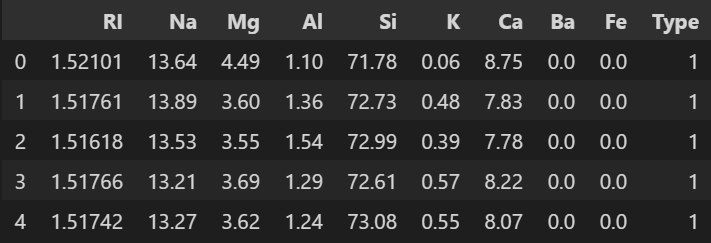
data = pd.read_csv("glass.csv")
 
# displaying the first five rows from the dataset
data.head()

You can also try this code with Online Python Compiler

Run Code

Output

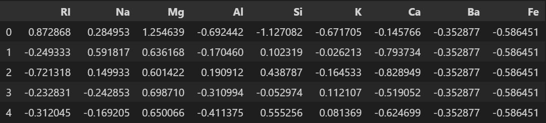
Pre-processing Data

from sklearn.preprocessing import StandardScaler
 
# Standardizing the features by removing the mean and scaling to unit variance.
scaler = StandardScaler()
 
# Computes the mean and std to be used for later scaling.
scaler.fit(data.drop('Type', axis=1))
 
# Perform standardization by centering and scaling.
scaled_features = scaler.transform(data.drop('Type', axis=1))
 
# constructing DataFrame
df_feat = pd.DataFrame(scaled_features, columns=data.columns[:-1])
 
# displaying the first five rows
df_feat.head()

You can also try this code with Online Python Compiler

Run Code

Output

Split the data into training and testing sets

from sklearn.model_selection import train_test_split
 
#Split data into random train and test subsets
X_train, X_test, y_train, y_test = train_test_split(scaled_features,data['Type'],test_size=0.30, random_state=42)

You can also try this code with Online Python Compiler

Run Code

Selecting the K value

from sklearn.neighbors import KNeighborsClassifier
 
error_rate = []
# Can take some time.
for i in range(1,10):
    # Classifier implementing the k-nearest neighbors vote.
    knn = KNeighborsClassifier(n_neighbors=i)
 
    # Fit the k-nearest neighbors classifier from the training dataset.
    knn.fit(X_train,y_train)
 
    # Now predicting the class labels for the X_test.
    predicted_i = knn.predict(X_test)
 
    error_rate.append(np.mean(predicted_i != y_test))

You can also try this code with Online Python Compiler

Run Code

Displaying the error rate for different values of K

plt.figure(figsize=(11,7))
plt.plot(range(1,10),error_rate,color='blue',linestyle='dashed', marker='o',markerfacecolor='red', markersize=8)
plt.title('Error Rate vs. K Value')
plt.xlabel('K')
plt.ylabel('Error Rate')

You can also try this code with Online Python Compiler

Run Code

Output

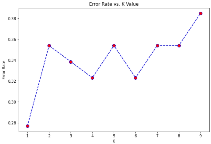
From the above plot, we can infer that the error rate is minimum at K=1. So we will choose k=1 for training our model.

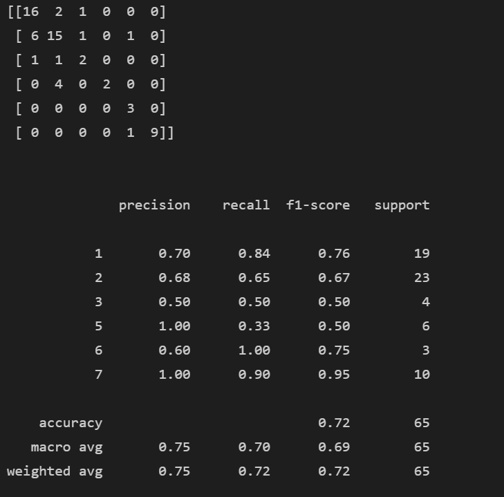
Model Prediction and Evaluation

# Classifier implementing the k-nearest neighbors vote.
knn = KNeighborsClassifier(n_neighbors=1)
 
# Fit the k-nearest neighbor classifier from the training dataset.
knn.fit(X_train,y_train)
 
# Now predicting the class labels for the X_test.
pred = knn.predict(X_test)

You can also try this code with Online Python Compiler

Run Code

from sklearn.metrics import classification_report,confusion_matrix
 
print(confusion_matrix(y_test,pred))
print('\n')
print(classification_report(y_test,pred))

You can also try this code with Online Python Compiler

Run Code

Output

You can find the complete code along with the dataset here. 

FAQs

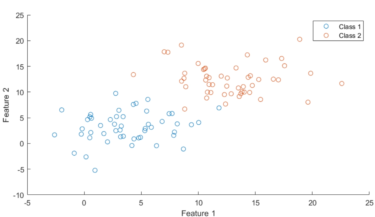
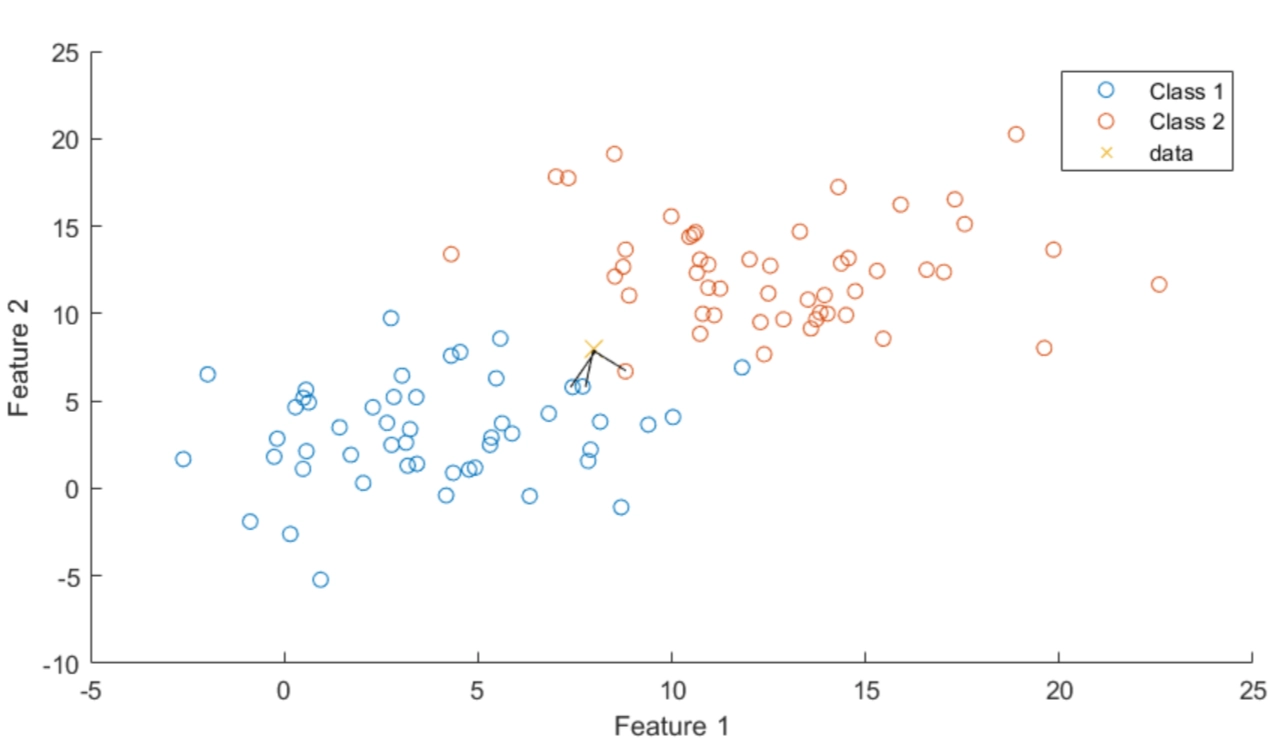
1. What is K in the KNN algorithm?
The number K in KNN refers to the number of nearest neighbors taken into account while giving a label to a datapoint.

2. What are the applications of this algorithm?
Applications of KNN include video recognition, image recognition, and handwriting detection. 
KNN is also the method behind most recommender systems.

Key Takeaways

Cheers if you reached here!! In this blog, we learned about the KNN algorithm. We saw its advantages, disadvantages, and its implementation too.

Yet learning never stops, For more information you may visit

https://www.codingninjas.com/courses/machine-learning

and there is a lot more to learn. 
Happy Learning!!