Limited-Memory Broyden-Fletcher-Goldfarb-Shanno Algorithm

BFGS algorithm

BFGS algorithm was discovered by four scientists named Broyden, Fletcher, Goldfarb, and Shanno.

• It is a local search algorithm done on purpose for convex optimization problems with a single optima.
• The BFGS algorithm belongs to a group of algorithms that is an extension to Quasi-Newton methods or Newton’s optimization method.
• Newton's optimization method is a second-order optimization algorithm that uses the Hessian matrix.

Newton's method requires the calculation of the inverse of the Hessian matrix. Calculating the Hessian matrix is computationally expensive and is not stable depending on the properties of the objective function. This is one of the limitations of Newton's method. Quasi-Newton methods are second-order optimization algorithms that approximate the inverse of the Hessian matrix using the gradient, meaning that the Hessian and its inverse do not need to be available or calculated precisely for each step of the algorithm.

L-BFGS algorithm

L-BFGS is an optimization algorithm and a so-called quasi-Newton method. Its name indicates that it's a variation of the Broyden-Fletcher-Goldfarb-Shanno (BFGS) algorithm, limiting how much gradient is stored in memory. By this, we mean the algorithm does not compute the full Hessian matrix, which is more computationally expensive.

L-BFGS approximates the inverse Hessian matrix to direct weight adjustments search toward more promising areas of parameter space. Whereas BFGS stores the gradient's full n × n inverse matrix, Hessian L-BFGS stores only a few vectors representing a local approximation. L-BFGS performs faster because it uses approximated second-order information. L-BFGS and conjugate gradient in practice can be faster and more stable than SGD methods.

Maths behind L-BFGS algorithm

IA second-degree approximation is used to find the minimum function f(x) in these methods. Taylor series of function f(x) is as follows:

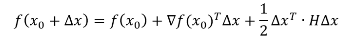
^Source

Here delta f is a function gradient, and H is hessian.

The Taylor series of the gradient will look like this:

Solving the equation to find the minimum.

Therefore we get:

Now hessian comes into play. Every method in this family has a different method of calling hessian.
You can also read about the memory hierarchy.

FAQ’s

1. Is BFGS gradient-based?
   The BFGS Hessian approximation can either be based on the full history of gradients, in which case it is referred to as BFGS, or it can be based only on the most recent m gradients, in which case it is known as limited memory BFGS, abbreviated as L-BFGS.
    
2. What is BFGS in machine learning?
   BFGS is a second-order optimization algorithm. It is an acronym named for the four co-discovers of the algorithm: Broyden, Fletcher, Goldfarb, and Shanno.
    
3. What are second-order optimization methods?
   Second-order optimization technique is the advance of first-order optimization in neural networks. It provides additional curvature information of an objective function that adaptively estimates the step-length of optimization trajectory in the training phase of the neural network.

Key Takeaways

In this article, we have discussed the following topics:

• Second-order optimization algorithm
• BFGS algorithm
• L-BFGS algorithm

Check out this article - Padding In Convolutional Neural Network
Hello readers, here's a perfect course that will guide you to dive deep into Machine learning.

Happy Coding!