Do you think IIT Guwahati certified course can help you in your career?
Introduction
Have you ever wondered how your email account accurately segregates regular emails, important emails, and spam emails? It’s not a very complex trick and we’ll learn the secret behind it. This is done with a supervised learning model called Logistic regression (However, it can be done with other machine learning algorithms also, but for the sake of this blog, we’ll stick to Logistic regression).
Logistic regression is employed in supervised learning tasks. More specifically, it is used for classification tasks. We know that name throws some people off. But the regression in the logistic regression is slightly misleading. It is NOT a regression model. Logistic regression is a probabilistic function. That means it makes use of probabilities of events to make its prediction.
Methodology
Suppose we are given a task, say we are given a customer’s banking history and are tasked to find if the customer can be sanctioned a loan. Basically we need to find if given a loan, will the customer default on payment or not. We can use logistic regression for this purpose. It will be a binary classification between ‘Yes’ or ‘No’. Logistic regression makes use of a sigmoid function and it is of the form -
We know the straight line equation -
y = w0 + w1x
We know the sigmoid function has a range between 0 and 1. So let’s divide the above equation by 1-y.
y / (1-y) : 0 for y = 0 and ∞ for y = 1
But we require our function to be between -∞ to +∞. For that, we’ll take logarithm so the new equation is:
Log (y / (1-y)) = w0 + w1x
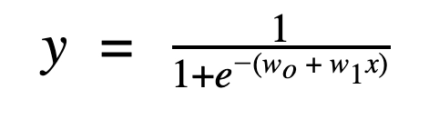
Upon simplifying our final equation then becomes -
Here y = predicted probability belonging to the default class( default class is 1(yes))
w0 + w1x = the linear model within logistic regression.
Also, the function is of the form of a sigmoid function
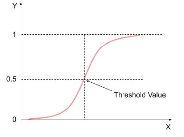
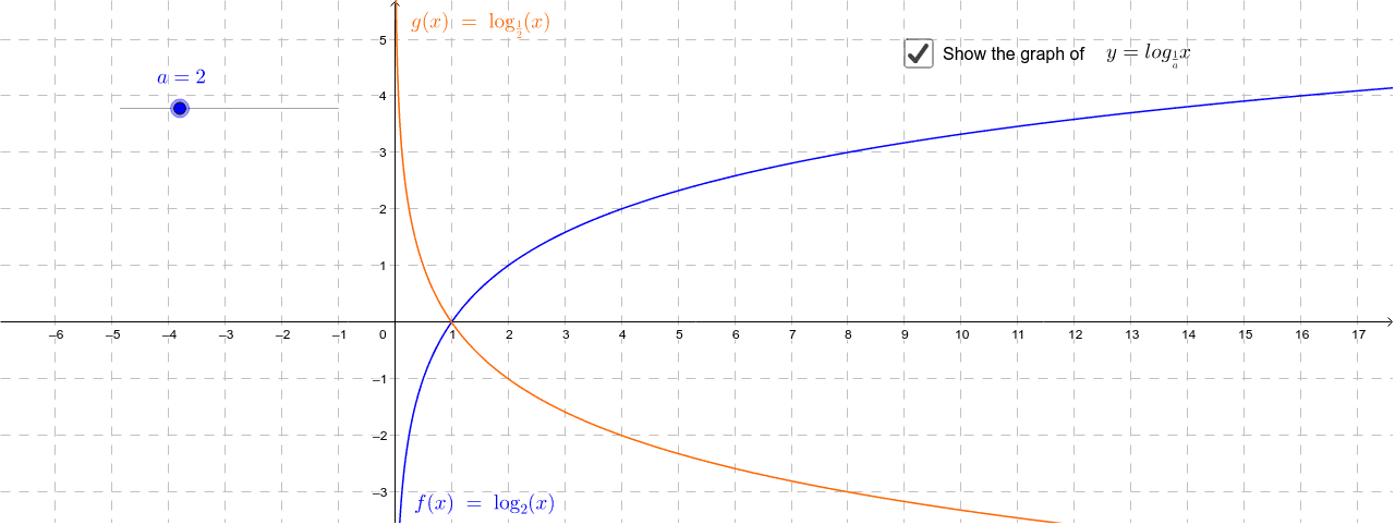
The Sigmoid function has a range between 0 and 1. And therefore forms an S-like curve.
The logistic function predicts the probability of an outcome. Hence its value lies anywhere between 0 and 1. And that’s where it gets its name from. We choose a threshold value above which the final prediction would be 1 and 0 otherwise.
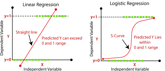
Let’s talk about the linear equation w0 + w1x within the logistic function. Why do we need the logistic regression function in the first place if it stems from linear regression?
It’s because the linear regression equation isn’t confined within a range, unlike logistic regression. And it would be a very difficult task to assign a threshold value for class membership for a linear regression function. Thus we feed the predicted value to a sigmoid function which makes it Logistic regression having a range between 0 and 1. Now since the range is between 0 and 1(no outliers) it would be convenient to do a probabilistic classification.
It represents a linear relationship between the input features and the final output.
Here x = input feature
w0 = bias term
w1 = weight associated with the input variable
Now suppose we take 0.5 as our threshold value. That means
A predicted value >0.5 from the logistic function would have the final prediction as 1 and,
A predicted value ≤0.5 from the logistic function would have the final prediction as 0.
Plotting the graph clears what makes logistic regression different from linear regression.
Cost Function
We know the cost function tells us how erroneous our model is. In the case of linear regression, our cost function was: -
Cost function =1/N ∑(y(i) - y(i)predicted )2
The linear regression cost function is used to find the average of errors in all predicted values corresponding to the actual value of y. But this cost function is suitable for logistic regression since logistic regression doesn’t have a continuous output variable, unlike linear regression. Suppose we were to use this cost function for a logistic regression model that does a binary classification(0 and 1). This would make the predicted value and the actual value either 0 or 1. This way we may end up at the local minima instead of the global minima. Remember, the cost function is minimum at the global minima.
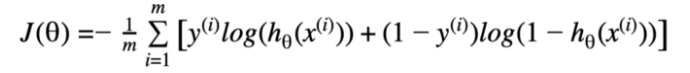
So we would require a new cost function for logistic regression. And it’s given below.
Here y(i) = the actual output for ith training example
hθx(i) = Predicted output for the ith training example by our model
Now we know that looks a bit overwhelming but let’s break it down term by term.
Suppose we train a logistic regression model and it correctly predicts the value 1.
So that means the predicted value of y would be closer to 1.
In this case, the second term in the logistic regression cost function becomes 0 (1-y = 1-1 = 0).
The first term would be-
y * log(ypredicted)= 1*log(~1) = ~0 ( low error)
Since the value is close to 1, therefore the cost function would compute a low error. Refer the log and -log graph given below.
Our predicted value was correct and therefore it makes sense for the error to be low.
In case had our model predicted 0 instead of 1, it would have led to a higher error since the log function for an input value closer to 0 would make our error exponentially high.
Gradient descent is a technique of altering the weights of data points based on the cost function. LogLoss cost function is calculated at each input-output data point.
We take a partial derivative with respect to bias and weight to find the slope of the cost function at every point.
Gradient descent then updates the values bias and weight values based on slope. This is an iterative process.
The iterations are done until the gradient descent reaches the minimum cost. The rate at which the gradient descent reaches the minima is called the learning rate.
Feature scaling is essential for gradient descent to work efficiently. We suggest you learn gradient descent in depth. You can refer to our blog on gradient descent if you wish to learn the math behind it.
Evaluating the model
Once we train the model it is necessary to evaluate how accurate our model really is. There are various evaluation metrics for this purpose.
Accuracy - It represents the number of correct predictions upon total number of predictions.
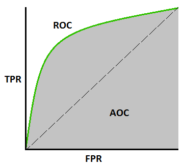
ROC AUC score - it stands for Receiver Operating Characteristic Curve. The area under the ROC AUC curve describes the relationship between the true positive rate (ratio of samples that were correctly predicted belonging to the correct class) and the false positive rate (the ratio of samples for which we incorrectly predicted their class membership). More area under the curve signifies better predictions, hence a better model.
We’ll start by importing the necessary libraries and the dataset. Here is the dataset. The dataset is about sales of a product via social media advertisement campaign. Our task at hand will be to predict if the item was purchased or not considering the given features.
import numpy as np
import pandas as pd
import matplotlib.pyplot as plt
from sklearn.model_selection import train_test_split
from math import exp
plt.rcParams["figure.figsize"] = (10, 6)
# Load the data
class LogisticRegression:
def __init__(self,datafile="Social_Network_Ads.csv"):
self.data = pd.read_csv(datafile)
self.data.head()
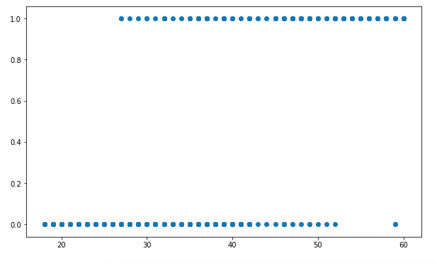
def PltFun(self):
plt.scatter(self.data['Age'], self.data['Purchased'])
plt.show()
# Split the training dataset and test dataset
def Training(self):
self.X_train, self.X_test, self.y_train, self.y_test = train_test_split(self.data['Age'], self.data['Purchased'], test_size=0.20,random_state=10)
def normalize(self):
self.X_train -= self.X_train.mean()
# Method to make predictions
def Sigmoid(self, b0, b1,x=None):
if x is None:
self.X_test-=self.X_test.mean()
return np.array([1 / (1 + exp(-1*b0 + -1*b1*i)) for i in self.X_test])
else:
return np.array([1 / (1 + exp(-1*b0 + -1*b1*i)) for i in x])
# Method to train the model
def logistic_regression(self):
# Initializing variables
self.normalize()
b0 = 0
b1 = 0
L = 0.001
epochs = 300
for epoch in range(epochs):
y_pred = self.Sigmoid(b0, b1,self.X_train)
D_b0 = -2 * sum((self.y_train - y_pred) * y_pred * (1 - y_pred)) # Derivative of loss wrt b0
D_b1 = -2 * sum(self.X_train * (self.y_train - y_pred) * y_pred * (1 - y_pred)) # Derivative of loss wrt b1
# Update b0 and b1
b0 = b0 - L * D_b0
b1 = b1 - L * D_b1
return b0, b1
def Accuracy(self , y_pred):
accuracy=0
for i in range(len(y_pred)):
if y_pred[i] == self.y_test.iloc[i]:
accuracy += 1
print(f"Accuracy = {accuracy / len(y_pred)}")
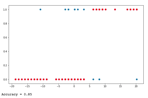
def Plot_result(self,y_pred):
plt.clf()
plt.scatter(self.X_test, self.y_test)
plt.scatter(self.X_test, y_pred, c="red")
plt.show()
def predictor(self,x):
x = [1 if p >= 0.5 else 0 for p in x]
return x
My_model = LogisticRegression()
My_model.PltFun()
My_model.Training()
b0,b1=My_model.logistic_regression()
y_pred = My_model.Sigmoid(b0,b1)
y_pred=My_model.predictor(y_pred)
My_model.Plot_result(y_pred)
My_model.Accuracy(y_pred)
You can also try this code with Online Python Compiler
What is a sigmoid function? Ans. The sigmoid function is given by 1 / ( 1 + e-z ) and its range is between 0 and 1.
Why is logistic regression called a probabilistic function? Ans. Logistic regression generates the probability of output given the input features. We then set a threshold value to classify the probability prediction.
Mention some real-life use cases of logistic regression. Ans. a. A bank can use a logistic regression model to predict if a customer would default on a loan b. A logistic regression model can be trained to tell if a tumour is benign or not.
Key takeaways
In this blog, we have thoroughly covered logistic regression. Its mathematical significance, its cost function, and its step-by-step python implementation. However, consider this a starting point. There is always room for improvement. If you want to ace your next data science interview, check out our machine learning courses curated by our faculty from Stanford University and industry experts.


 6+ registered

