Table of contents

Introduction

Hypothesis

Cost Function

Regularization

Optimization

Implementation

5.1.

Python

Frequently Asked Questions

6.1.

What is the difference between cost function and loss function in logistic regression?

6.2.

Why not MSE as a loss function for logistic regression?

6.3.

What loss function is used for logistic regression?

6.4.

How to choose a loss function?

6.5.

Which cost function is used for logistic regression?

Conclusion

Last Updated: May 24, 2024

Easy

Loss Function for Logistic Regression

Q: What is the difference between cost function and loss function in logistic regression?

The loss function measures the error for a single training example, while the cost function is the average of the loss functions over all training examples. In logistic regression, the cost function is the mean of the loss calculated by the logistic loss (log loss or cross-entropy loss) across the entire dataset.

Q: Why not MSE as a loss function for logistic regression?

Mean Squared Error (MSE) is not suitable for logistic regression because it assumes a continuous output and a linear relationship between input and output. Logistic regression deals with binary outcomes, and MSE can lead to non-convex cost functions, making optimization more challenging.

Q: What loss function is used for logistic regression?

The loss function used in logistic regression is log loss (logistic loss or cross-entropy loss). It measures the performance of a classification model whose output is a probability value between 0 and 1, penalizing incorrect classifications more heavily.

Q: How to choose a loss function?

Choosing a loss function depends on the problem type. For regression, use MSE or MAE. For binary classification, use log loss. For multiclass classification, use categorical cross-entropy. The loss function should align with the model’s objective and the nature of the target variable.

Q: Which cost function is used for logistic regression?

The cost function for logistic regression is the average of the log loss over all training examples. It is often referred to as the cross-entropy cost function and is designed to optimize the parameters to minimize the prediction error for binary classification tasks.

Author soham Medewar

Do you think IIT Guwahati certified course can help you in your career?

Yes

Introduction

The first topic that we learn while diving into machine learning is linear Regression, and next to it is logistic Regression. Before getting started on the topic, I recommend you recall the topics of linear Regression.

Let us just quickly revise the logistic regression. Logistic regression is a classification algorithm in supervised learning used to find the probability of a target variable. In simple words, the output of a model is binary(either 0 or 1). Examples of classification problems are online transaction fraud or not fraud, email spam or not, checking whether a person has cancer or not.

All these types of classification lie under logistic regression.

So, what will be the loss function for the above classification problems? In the article below, I will be explaining the loss function used in logistic regression.

Hypothesis

Firstly, I will define a hypothesis for the linear regression.

h𝝷(x) = 𝝷₀x₀+𝝷₁x₁+𝝷₂x₂+ ... +𝝷ₙxₙ=[𝝷₀+𝝷₁+𝝷₂+ ... +𝝷ₙ]

Where x₀ = 1

Let us Define this hypothesis function of linear Regression as raw model output. In logistic Regression, we have transformed the above hypothesis function. In logistic Regression, we mainly do binary classification based on the output, i.e., 1 or 0. But there are some problems with the hypothesis function of linear Regression; we have to transform it so that its output lies between 0 to 1. If we look onto a sigmoid function for all values of its output lies between 0 to 1. So for the hypothesis function of Logistic Regression, we use the sigmoid function as shown below.

Sigmoid function:

Hypothesis function:

Graph of the hypothesis function.

In the above graph, we can see that for all values of the x hypothesis function lies between 0 to 1.

The output of the above hypothesis function tells the probability of y=1. For given x, parameterized by θ, hypothesis h(x) = P(y = 1|x; θ).

We can describe decision boundary as: Predict 1, if θᵀx ≥ 0 → h(x) ≥ 0.5; Predict 0, if θᵀx < 0 → h(x) < 0.5.

Cost Function

Let us remember the loss function of Linear Regression; we used Mean Square Error as a loss function as the figure below shows the graph of the loss function of linear Regression.

MSE = (1/n) *∑ (y - Ŷ)²

Here y - Ŷ is the difference between actual and predicted value.

When the Gradient Descent Algorithm is applied, all the weights will be adjusted to minimize error.

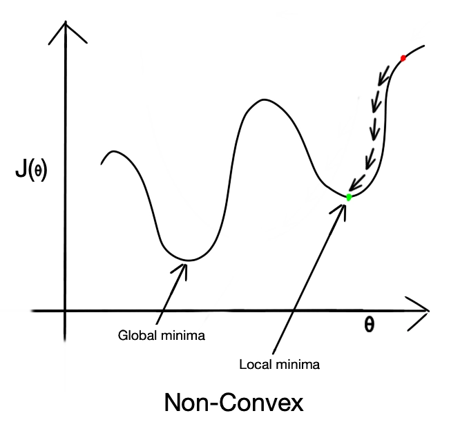
But in the case of Logistic Regression, we cannot use Mean Squared Error as a loss function because the hypothesis function of logistic is non-linear. Suppose we apply Mean Squared Error as a loss function. In that case, we will get many local minima, and Gradient Descent Algorithm cannot minimize the error as it gets terminated at local minima. The non-linearity introduced by the sigmoid function in the hypothesis causes the non-convex nature of Mean Squared Error with logistic Regression. Relation between weighted parameters and error becomes complex.

Another reason for not using Mean Squared Error in Logistic Regression is that our output lies between 0 - 1. In classification problems, the target value is either 1 or 0. The output of the Logistic Regression is a probability value between 0 to 1. The error (y - p)² will always be between 0-1. Therefore tracking the progress of error value is difficult because storing high precision floating numbers is challenging, and we also cannot round off the digits.

Due to the above reasons, we cannot use Mean Squared Error in logistic Regression.

Intuitively, we want to assign more punishment when predicting 0 while the actual is 1 and when predicting 1 while the actual is 0. While making loss function, there will be two different conditions, i.e., first when y = 1, and second when y = 0.

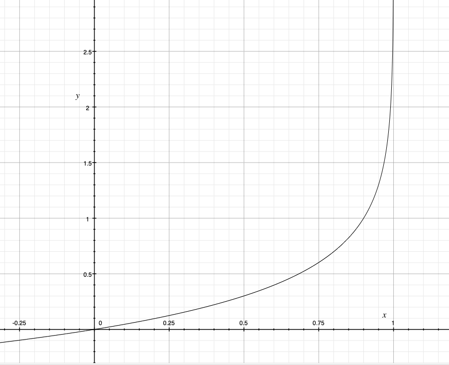
The above graph shows the cost function when y = 1. When the prediction is 1, we can see that the cost is 0. When the prediction is 0, the cost is 1. Therefore, a high cost punishes the learning algorithm. (x-axis represents h𝝷(x) predicted value and the y-axis represents cost)

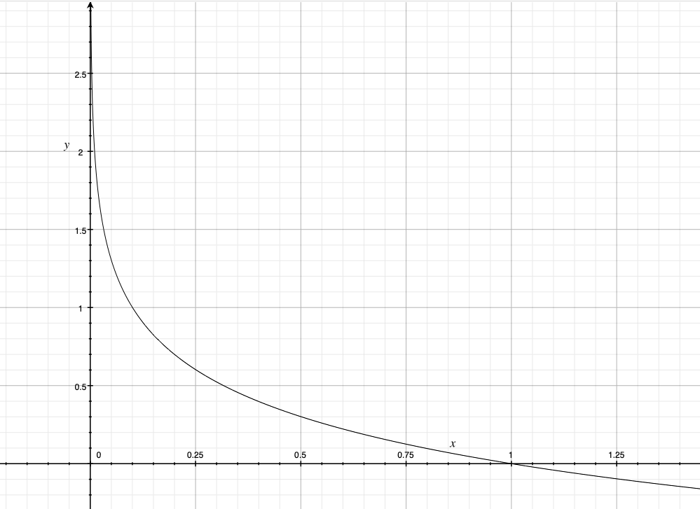
The above graph shows the cost function when y = 0. When the prediction is 1, we can see that the cost is 1; therefore, a high cost punishes the learning algorithm. (x-axis represents h𝝷(x) predicted value and the y-axis represents cost)

Therefore the cost function can be defined as

Image source

Combining the equation for y=1 and y=0, we get the following equation.

Image source

The cost function for the model will be a summation of all the training points.

Image source

Regularization

Regularization in logistic regression is a technique used to prevent overfitting by adding a penalty to the loss function. Overfitting occurs when the model learns not only the underlying pattern but also the noise in the training data, leading to poor performance on unseen data.

There are two common types of regularization used in logistic regression:

L1 Regularization (Lasso)
L2 Regularization (Ridge)

Optimization

Optimization in logistic regression involves finding the set of parameters (weights 𝑤w) that minimize the loss function. The loss function measures how well the model's predictions match the actual data. In the context of logistic regression, the loss function is often the negative log-likelihood (or cross-entropy loss), which is convex and hence has a single global minimum.

Common optimization algorithms used for logistic regression include:

Gradient Descent
Newton's Method
Quasi-Newton Methods (e.g., BFGS)
Conjugate Gradient Method

Implementation

We will see the code for the above-discussed loss function in this part.

Python

Python

## Vectorized Implementation of Optimization Using Gradient Descent
# Define first derivative of cost function
def cost_dev(j, t, X=X, y=y, m=m):
  dev = X[:, j]@(1/(1 + np.exp(-X@theta)) - y)
  dev = (1/m)*dev
  return dev

# Define Cost function
def cost(t, h, l=l, X=X, y=y, m=m):
  cost = np.transpose(-y)@np.log(h) - np.transpose(1-y)@np.log(1-h) + (l/2)*np.transpose(t[1:])@t[1:]
  cost = (1/m)*cost
  return cost
# Define iterations

theta_temp = np.zeros(theta.shape)
cost_list = []
theta_list = []
for i in range(1000000):
  for j in range(len(theta)):
      if j == 0:
          theta_temp[j] = theta[j] - a*cost_dev(j, theta)
      else:
          theta_temp[j] = theta[j]*(1 - (a*lmbd)/m) - a*cost_dev(j, theta)
  
  theta = theta_temp       
  hypo = 1/(1 + np.exp(-X@theta))
  
  theta_list.append(list(theta))
  cost_val = cost(theta, hypo)
  cost_list.append(cost_val)

You can also try this code with Online Python Compiler

Run Code

Frequently Asked Questions

What is the difference between cost function and loss function in logistic regression?

The loss function measures the error for a single training example, while the cost function is the average of the loss functions over all training examples. In logistic regression, the cost function is the mean of the loss calculated by the logistic loss (log loss or cross-entropy loss) across the entire dataset.

Why not MSE as a loss function for logistic regression?

Mean Squared Error (MSE) is not suitable for logistic regression because it assumes a continuous output and a linear relationship between input and output. Logistic regression deals with binary outcomes, and MSE can lead to non-convex cost functions, making optimization more challenging.

What loss function is used for logistic regression?

The loss function used in logistic regression is log loss (logistic loss or cross-entropy loss). It measures the performance of a classification model whose output is a probability value between 0 and 1, penalizing incorrect classifications more heavily.

How to choose a loss function?

Choosing a loss function depends on the problem type. For regression, use MSE or MAE. For binary classification, use log loss. For multiclass classification, use categorical cross-entropy. The loss function should align with the model’s objective and the nature of the target variable.

Which cost function is used for logistic regression?

The cost function for logistic regression is the average of the log loss over all training examples. It is often referred to as the cross-entropy cost function and is designed to optimize the parameters to minimize the prediction error for binary classification tasks.

Conclusion

In this article, we have discussed Logistic Regression for loss function. Furthermore, we discussed why the loss function of linear Regression could not be used in logistic Regression. Some important derivations and implementation of the loss functions were covered in this article.

Hello readers, here's a perfect course that will guide you to dive deep into Machine learning.

Happy Coding!