Table of contents
1.
Introduction
2.
Problem Statement
2.1.
Sample Examples
3.
Approach
3.1.
Algorithm
3.2.
Implementation in Java
3.3.
Implementation in C++
3.4.
Complexity Analysis
4.
Frequently Asked Questions
4.1.
Which data structure is used to form a Matrix? Explain it.
4.2.
What is the need for a two-dimensional array?
4.3.
How are two-dimensional arrays stored in memory?
4.4.
How can we obtain data from a two-dimensional array?
5.
Conclusion
Last Updated: Mar 27, 2024
Medium

Matrix probability problem

Author Rupal Saluja
0 upvote
Career growth poll
Do you think IIT Guwahati certified course can help you in your career?

Introduction

In this blog, we will try to grab hold of a two-dimensional array data structure problem. The problem aims to find the probability of an element of a matrix crossing the boundaries when moved by n positions.

Representation of 2-D Array

Through this problem, we will try to understand how to approach any two-dimensional array data structure problem. We will learn about two-dimensional data structure and examine the problem statement. The examples presented will help you clear your concepts, the algorithm will provide you with an immediate solution, and the implementation part will give you a detailed understanding of every step.

Notion of Coding

Also Read About, Array Implementation of Queue and  Rabin Karp Algorithm

What is Matrix?

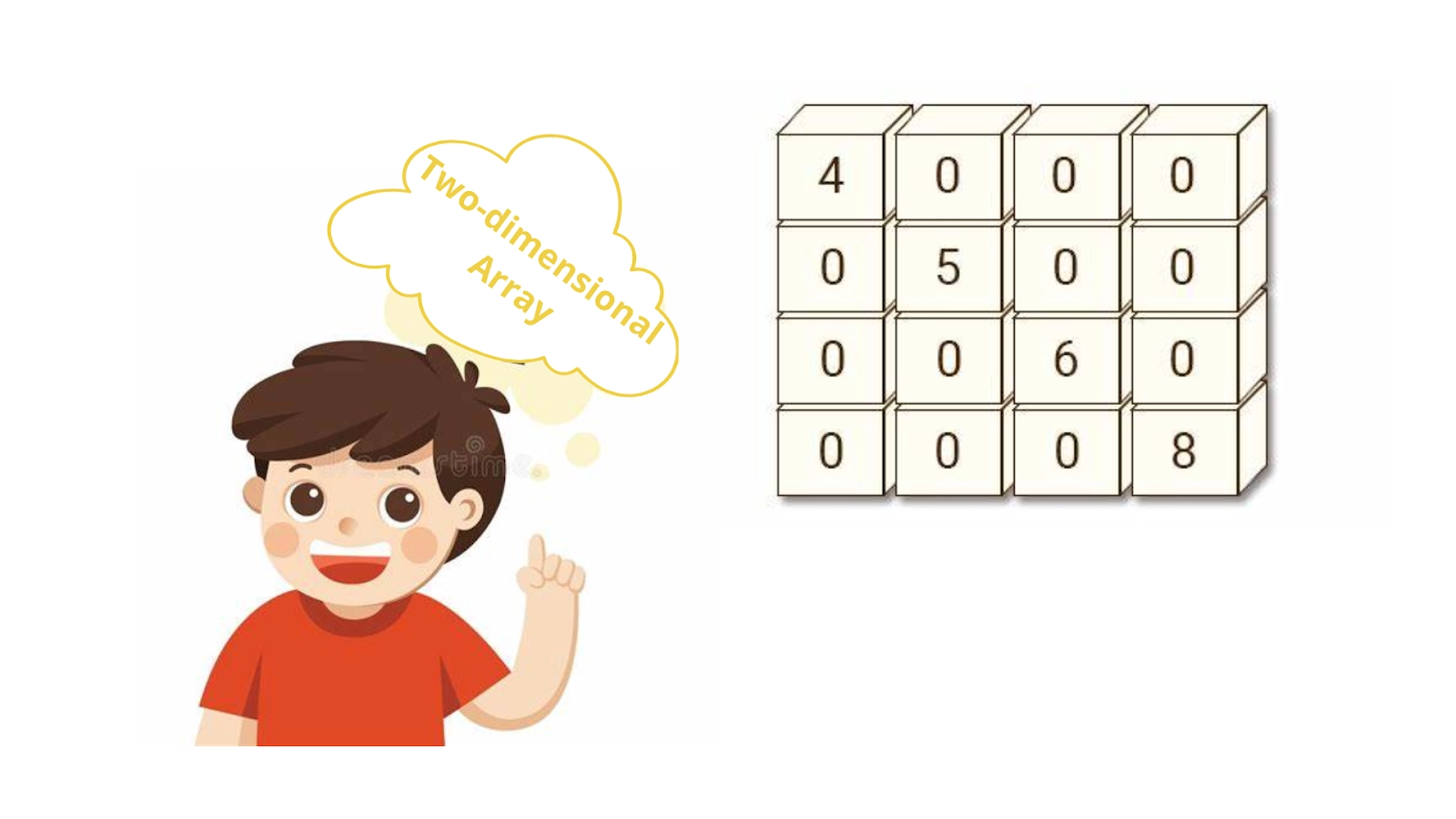
A matrix can be made using a two-dimensional array data structure. A multidimensional array is an array within arrays. That is, each element of the multidimensional array is an array itself. Similarly, in a two-dimensional array, every element of an array is an array in itself. 

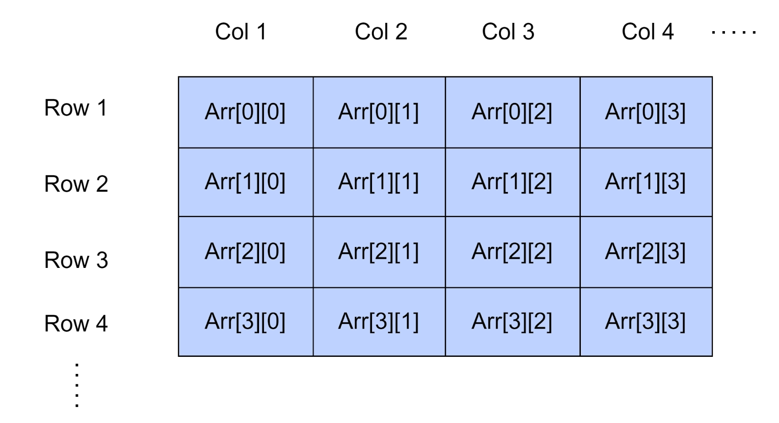
For example, we use the following line of Java code to create a multidimensional array presented below.

int [][] a= new int [3][4];

This two-dimensional array can store up to 12 elements.

Two-Dimensional Array

Problem Statement

Firstly, we will have a look at what exactly the problem says.

We are given a matrix of a random order. We need to output the probability for any given vertex of a matrix that, when moved by n positions, never crosses any boundary. 

The current cell can move in four directions, left, right, top, or bottom, with equal probability. Here, we have assumed that no index in the matrix remains empty and all the indices have some value. There are no exceptions to this problem.

To understand all the possible cases better, we have used the matrix of the same order in all the examples.

Sample Examples

🍇 Example 1: When a vertex is invalid.

Input: i = 4, j = 4 (Order of Matrix)

          x = 5, y = 3 (Coordinates of the Vertex)

          n = 3 (Shift in position)

Output: 0.0

Explanation:

In the example above, you will observe a matrix of order 4*4. The input x and y added as coordinates of the vertex are not present inside the matrix boundary. This makes the vertex invalid. If the vertex is invalid, that is, outside the matrix boundary, its probability of crossing any boundary automatically becomes zero. This output is irrespective of whatever we input as a shift in position.


🍇 Example 2: When a vertex is valid, but there is no shift in position.

Input: i = 4, j = 4 (Order of Matrix)

          x = 2, y = 3 (Coordinates of the Vertex)

          n = 0 (Shift in position)

Output: 1.0

Explanation:

In the example above, you will observe a matrix of order 4*4. The input x and y added as coordinates of the vertex are present inside the matrix boundary. This makes the vertex valid. Now, as the shift in position is zero and we already know that the vertex is inside the matrix boundary, its probability of remaining inside the boundary automatically becomes one. This output completely depends on the input added as a shift in position.


🍇 Example 3: When a vertex is valid, and position shift is equal to 3.

Input: i = 4, j = 4 (Order of Matrix)

          x = 2, y = 3 (Coordinates of the Vertex)

          n = 3 (Shift in position)

Output: 0.453125

Explanation:

In the example above, you will observe a matrix of order 4*4. The input x and y added as coordinates of the vertex are present inside the matrix boundary. This makes the vertex valid. Now, as you can see, the shift in position is three, so the output is calculated based on the algorithm, with no exceptions. This output depends on the input added as a shift in position and on the vertex.


🍇 Example 4: When the vertex is valid, and the matrix has been crossed completely.

Input: i = 4, j = 4 (Order of Matrix)

          x = 4, y = 4 (Coordinates of the Vertex)

          n = 2 (Shift in position)

Output: 0.0

Explanation:

In the example above, you will observe a matrix of order 4*4. The input x and y added as coordinates of the vertex are present on the matrix boundary. This makes the vertex valid. But, as you can see, the vertex is on the verge of crossing the boundary, so any value greater than zero for a shift in position would result in the vertex crossing the boundary. Thus, the probability becomes zero. This output depends on the input added as a shift in position and on the vertex.

Approach

The approach is somewhat similar to Depth First Search (DFS Algorithm). Firstly, we will check the validity of the given vertex. If the matrix is invalid or has crossed the boundaries, the output straight away equals 0. If there is a surety that even after moving n steps, no boundaries would be crossed, that is, n is 0, then 1 will be the output.

We perform recursive traversing in each direction for each cell that comes in the way, w. As per the problem statement, each direction has an equal probability, so each direction will contribute ¼ of the total probability of that particular cell, that is, 0.25. The required probability is calculated with one less move so that necessary steps can be taken in case of an exception, such as stepping out of the matrix.

Algorithm

Prob(int i, int j, int x, int y, int n)

i,j = Order of Matrix

x,y = Coordinates of vertex

n = Shift in position

Start
   if x, y is not present inside matrix boundary i, j, return 0
   if n = 0 , return 1
   double prob = 0
   prob = prob + matProb(m, n, x-1, y, N-1) * 0.25
   prob = prob + matProb(m, n, x+1, y, N-1) * 0.25
   prob = prob + matProb(m, n, x, y+1, N-1) * 0.25
   prob = prob + matProb(m, n, x, y-1, N-1) * 0.25
   return prob
End

Implementation in Java

import java.io.*;
class Main
{
    public static void main (String[] args)
    {
        int i = 3, j = 4;
        int x = 2, y = 2;
        int n = 3;
        System.out.println(Prob(i, j, x, y, n));
    }
    static boolean Validity(int a, int b, int i, int j)
    {
        return (a >= 0 && a < i && b >= 0 && b < j);
    }
    static double Prob(int i, int j, int a, int b, int n)
    {
        if (! Validity(a, b, i, j))
            return 0.0;
        if (n == 0)
            return 1.0;
        double p = 0.0;
        p += Prob(i, j, a - 1, b, n - 1) * 0.25;
        p += Prob(i, j, a, b + 1, n - 1) * 0.25;
        p += Prob(i, j, a + 1, b, n - 1) * 0.25;
        p += Prob(i, j, a, b - 1, n - 1) * 0.25;
        return p;
    }
}

Implementation in C++

#include <bits/stdc++.h>
using namespace std;
bool Validity(int a, int b, int x, int y)
{
    return (a >= 0 && a < x && b >= 0 && b < y);
}
double Prob(int x, int y, int a, int b, int n)
{
    if (!Validity(a, b, x, y))
        return 0.0;
    if (n == 0)
        return 1.0;
    double p = 0.0;
    p += Prob(x, y, a - 1, b, n - 1) * 0.25;
    p += Prob(x, y, a, b + 1, n - 1) * 0.25;
    p += Prob(x, y, a + 1, b, n - 1) * 0.25;
    p += Prob(x, y, a, b - 1, n - 1) * 0.25;
    return p;
}
int main()
{
    int x = 3, y = 4;
    int i = 2, j = 2;
    int n = 3;
    cout << Prob(x, y, i, j, n);
    return 0;
}


Input:

i=3, j=4, x=2, y=2, n=3


Output:

0.4375

Complexity Analysis

🌾 Time Complexity:

As you can see, no loops have been used, and the implementation seems simple. Hence we conclude that the time complexity for the code mentioned above will be: O(n).

🌾 Space Complexity:

Also, no extra space has been used in the solution above. Thus, the space complexity for the code mentioned above will be O(1).

Frequently Asked Questions

Which data structure is used to form a Matrix? Explain it.

A two-dimensional array is a data structure used to form a Matrix. Arrays within the arrays are called two-dimensional arrays, which are collections of rows and columns.

What is the need for a two-dimensional array?

Data that cannot be stored in a single-dimensional array, that is, the information that requires rows and columns to be stored, managed, and assessed in a one-dimensional array, are stored in two-dimensional arrays.

How are two-dimensional arrays stored in memory?

A two-dimensional array in the form of one row following another in the computer’s memory.

How can we obtain data from a two-dimensional array?

Like a one-dimensional array, we can obtain data from any individual cell of a two-dimensional array by using the indices of the cells. In two-dimensional arrays, two indices are attached to each cell. One index denotes row number, while the other denotes column number.

Conclusion

In a nutshell, we looked at the problem statement, had a look at every possible condition that could occur, understood the approach, went through the Algorithm, saw the implementations, tested the code against sample input, and did time and space complexities’ analysis.

We hope the above discussion helped you understand and solve the problem better, and now it is your turn to code the problem in your way.

For enthusiasts who want to solve more such questions, refer to the list below.


Enroll in our courses, go for mock tests, solve problems available, and interview puzzles. Also, you can focus on interview stuff- interview experiences and an interview bundle for placement preparations. Do upvote our blog to help other ninjas grow.

Happy Coding!

Live masterclass