Do you think IIT Guwahati certified course can help you in your career?
Introduction
Array is one of the first Data Structures that we learn while learning any of the programming language concepts. It is one of the most useful and elementary data structures. In the following article, we discuss a problem involving arrays ‘Maximize Score by Multiplying Elements of Given Array with Given Multipliers’ following from most intuitive to to most optimal approach and their analysis.
Problem Statement
We are given two arrays ARR[] and MUL[] of length 'N' and 'M' respectively, where N >= M. We need to iterate through the multiplier array (MUL[]) and for every element MUL[i], we need to pick an element from ARR[], either from the start or the end such that the sum of their products is maximized.
Example1
Input
ARR[] = {5, 6, 7}
MUL[] = {7, 6, 5}
Output
110
Explanation
Choose from the end, add 7 * 7, i.e. 49, to the result. Next, choose from the end, add 6 * 6, i.e. 36, to the result. Finally, choose from the end and add 5 * 5, i.e. 25, to the result. RESULT = 49 + 36 + 25 = 110
Example2
Input
ARR[] = {8, 7}
MUL[] = {0}
Output
0
Explanation
No matter we choose from start or end, we will get 0 as the value of the multiplier is 0.
Naive Solution
Idea
The idea is pretty simple. We will explore every possibility recursively (see Recusrion) and return the maximum. For this, we need to traverse through the multiplier array (MUL) and for every element MUL[i] we have two choices, either pick an element from the start of the array or the end of the array and multiply it with the multiplier, add to the result of the subproblem, compare both results and return the maximum of the two.
Algorithm
To solve this problem, we define a function getMaxScore(ARR, MUL, L, R, I). This function returns the maximum score we can achieve from the subarray { ARR[L], ARR[L+1], ARR[L+2]...ARR[R] } and { MUL[I], MUL[I+1], MUL[I+2]..., MUL[M - 1] }.
We define the function getMaxScore(ARR, MUL, L, R, I) as follows:
When I == M, the base case return 0. When we don’t have any elements left in the multiplier array, we simply return 0.
Otherwise, we return the maximum of :
ARR[L] * MUL[I] + getMaxScore(ARR, MUL, L + 1, R, I + 1) i.e. chose element from the start of the array.
ARR[R] * MUL[I] + getMaxScore(ARR, MUL, L, R + 1, I + 1) i.e. chose element from the end of the array.
Note that we are recursively calling for getMaxScore(ARR, MUL, L + 1, R, I + 1) and getMaxScore(ARR, MUL, L, R + 1, I + 1) and using their solution to build our final solution.
C++ Code
#include <bits/stdc++.h>
using namespace std;

int getMaxScore(vector<int> &arr, vector<int> &mul, int l, int r, int i)
{
  int n = arr.size(), m = mul.size();

  // Base case
  if (i == m) {
      return 0;
   }

  // Pick from the start or pick from the end
  return max(arr[l] * mul[i] + getMaxScore(arr, mul, l + 1, r, i + 1), arr[r] * mul[i] + getMaxScore(arr, mul, l, r - 1, i + 1));
}

// Driver Code
int main()
{

  vector<int> array = {5, 6, 7};
  vector<int> multipliers = {7, 6, 5};

  cout << getMaxScore(array, multipliers, 0, array.size() - 1, 0) << endl;

  return 0;
}
You can also try this code with Online C++ Compiler
There are M elements in the multiplier array. For every element MUL[I], we have two choices: select an element from the start or the end of the array, multiply it with the MUL[i], and add it to the result of the subproblem. Hence the time complexity is O(2M).
Space Complexity: O(1)
We are not using any auxiliary space; hence the space complexity is O(1).
Efficient solution
Idea
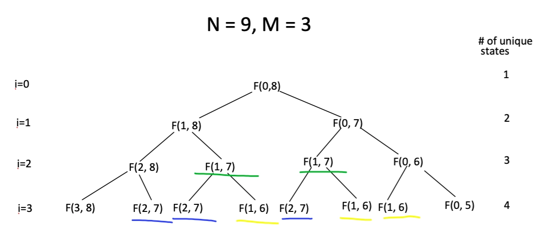
We will use dynamic programming to solve this problem efficiently; specifically, we will be using memoization. We are using dp because this problem has optimal substructure and overlapping subproblems, clearly seen from the image attached below. Equivalent states are underlined with the same color (Also see DP with Arrays)
Algorithm
We define some global variables, DP[1000][1000] = -1, a 2D DP array to store the solution of subproblems.
ARR[] and MUL[] (input arrays), just to decrease the number of parameters in the getMaxScore function. In the image above, F = getMaxScore.
Finally, we define the getMaxFunction(L, R). It takes two arguments, L and R, which defines our subarray { ARR[L], ARR[L+1], ARR[L+2] … ARR[R] }. This function returns the maximum score that can be obtained from this subarray.
N = size of “ARR”, M = size of multiplier array “MUL”.
IDX points to the current multiplier, i.e. MUL[IDX]. We can observe that IDX is a function of L, R. IDX = N - (R - L + 1). This relation can be deduced from the fact that the number of elements in the subarray, i.e. ARR[L], ARR[L+1], ARR[L+2] … ARR[R] is R - L + 1. So the number of multipliers already taken is N - (R - L + 1). Hence the current multiplier is MUL[IDX].
Check for the base case, i.e. when IDX == M, we set and return DP[L][R] = 0.
The figure above shows that the value IDX(=i) goes from 0 to M. Hence the total number of levels in the recursion tree is M + 1. This observation is crucial to analyse the time complexity.
We then check if this subproblem is already solved, i.e. if DP[L][R] != -1, we return DP[L][R].
Otherwise, we calculate and return DP[L][R] that is equal to maximum of:
ARR[L] * MUL[IDX] + getMaxScore(L + 1, R), choosing from the start
ARR[R] * MUL[IDX] + getMaxScore(L, R - 1), choosing from the end
C++ Code
#include <algorithm>
using namespace std;

int dp[1000][1000];
vector<int> arr, mul;

int getMaxScore(int l, int r)
{
   int n = arr.size(), m = mul.size();

   //  idx is a function of n, m
   int idx = n - (r - l + 1);

   // Checking for the base case
   if (idx == m)
   {
       return dp[l][r] = 0;
   }

   // Checking if the dp state is already calculated
   if (dp[l][r] != -1)
   {
       return dp[l][r];
   }

   /*
   Return the maximum of the two possibilites i.e.
   pick an element from the start of the array
   or the end of the array.
   */
   return dp[l][r] = max(mul[idx] * arr[l] + getMaxScore(l + 1, r), mul[idx] * arr[r] + getMaxScore(l, r - 1));
}

// Driver code
int main()
{
   memset(dp, -1, sizeof(dp));
   arr.clear(), mul.clear();

   // Example input
   arr = {5, 6, 7};
   mul = {7, 6, 5};
   cout << getMaxScore(0, arr.size() - 1) << endl;
   return 0;
}
You can also try this code with Online C++ Compiler
The total number of unique DP states = (M+1)(M+2)/2. This can be shown from the image above. In the above image, we have a recursion tree and multiple levels in it. Every level has one more unique state than the previous one (starting from one). The total number of levels = M + 1. Hence, total number of unique states = 1 + 2 + 3 + … + (M + 1) = (M+1)(M+2)/2. Calculating the value of a DP state requires constant time hence the overall time complexity is O(M2).
We are using an auxiliary DP array to store the value of subproblems. The maximum number of rows and columns in the DP array is N because, L can range from [0, M] and R can range from [N - M - 1, N - 1].
If the problem possesses the following properties, then we can use dp: Optimalsubstructure: Optimal solution of a bigger problem can be calculated using optimal solution(s) of smaller subproblem(s). Overlapping subproblems: Some subproblems may have some common states which need to be evaluated. Instead of calculating those states multiple times, we calculate it once and store the value and use it whenever required, hence reducing the computation time.
Can we optimize the space complexity?
Yes, we can reduce the space complexity from O(N2) to O(M2), because essentially there is (M+1)(M+2)/2 number of states. So, to store the DP states we need O(M2) space.
Conclusion
In this blog, we solved an interesting optimization problem using dynamic programming. We solved it using two approaches. First was a basic recursion based approach which took exponential time, whereas the efficient solution was bottom-up DP based, which took polynomial time. We also discussed when to use dp and what is the difference between the top-down and bottom-up approaches.


 9+ registered

